Gradient-Oriented Boundary Profiles for Shape Analysis Using Medial Features
This research focuses on developing advanced boundary detection methods for shape analysis, particularly in the context of cardiovascular disease diagnosis through medical imaging. The study presents a systematic approach to extracting gradient-oriented boundary profiles, validating their effectiveness, and applying them to shape analysis routines, with a focus on real-time 3D ultrasound data.

Gradient-Oriented Boundary Profiles for Shape Analysis Using Medial Features
E N D
Presentation Transcript
Gradient-Oriented Boundary Profiles for Shape Analysis Using Medial Features Robert J. Tamburo, BS Bioengineering University of Pittsburgh Under the Advisement of: George D. Stetten, MD, PhD U. Pitt. Bioengineering CMU Robotics Institute
Overview • Background Part I • Gradient-Oriented Boundary Profiles • Validation of Boundary Profiles • Background Part II • Boundary Profiles and Shape Analysis • Results on Synthetic and RT3D Ultrasound Data • Future Work • Conclusion
Clinical Motivation • In 1999: • Cardiovascular Disease (CVD) contributed to one-third of worldwide deaths • CVD ranks as the leading cause of death in the U.S. responsible for 40% of deaths per year • 62 million Americans live with some form of cardiovascular disease • Americans were expected to pay about $330 billion in CVD-related medical costs this year *CDC/NCHS and the American Heart Association Causes of Death for All Americans in the United States, 1999 Final Data
Image Analysis • Left ventricular (LV) and myocardial volume to calculate cardiac function parameters: - cardiac output - stroke volume - ejection fraction • Myocardial thickness and motion can be monitored • Diagnoses of CVD, including cardiomyopathy, arrhythmia, ischemia, valve disease, myocardial infarction, and congestive heart failure
Medical Imaging • 2D ultrasound • 3D ultrasound • Gating to the electrocardiogram • Mechanically scanned • Cine-CT • 50 ms/slice (400 ms for full volume) • Real-time three-dimensional (RT3D) ultrasound • 22 frames/sec (45 ms)
Goals • Automatically identify and measure structures RT3D ultrasound data • Develop “intelligent” boundary points: Gradient-Oriented Boundary Profiles • Apply to Profiles to a shape analysis routine
Boundary Detection • First step in most Image Analysis routines • Convolution with kernel in spatial domain • High-pass frequency filters in frequency domain • Spatial domain detection: • is computationally less expensive • often yields better results
Gradient Based Detectors • Gradient magnitude is rotationally insensitive • Gradient magnitude sensitive to: • object intensity • background intensity • overall image contrast
Common Gradient Based Detectors • Roberts Cross • 2x2 kernel • Very sensitive to noise • Very fast • Sobel • 3x3 kernel • Somewhat sensitive to noise • Slower than Roberts Cross • Both amplify high-frequency noise (derivative)
GradientBasedBoundary Detectors With Smoothing • Marr • Gaussian Smoothing • Laplacian of Gaussian • Canny • Gaussian smoothing • Ridge tracking • Both require multiple applications • Some fine detail lost
Algorithm for Classifying Boundaries • Find candidate boundary points • Create an intensity profile • Fit a cumulative Gaussian to the intensity profile • Eliminate blatantly “bad” profiles • Calculate measures of confidence • Classify the boundary
Difference of Gaussian (DoG) Detector • Gradient magnitude • Gaussian smoothing • Difference between 3 same-scale Gaussian kernels • Measures gradient direction components in 3D
Finding Candidate Boundary Points • Over sample with small sampling interval • Apply gradient detector (DoG) • Accept those above pre-determined threshold
Algorithm for Classifying Boundaries • Find boundary candidates • Create an intensity profile • Fit a cumulative Gaussian to the intensity profile • Eliminate blatantly “bad” profiles • Calculate measures of confidence • Classify the boundary
Generating an Intensity Profile • Sample voxels in a neighborhood • Partition sampling region • Project voxels (splat) to the major axis
Sampling Voxels • Ellipsoidal or cylindrical • Centered at boundary point • Major axis in direction of gradient • Reduces the effect of image noise
Splatting Voxel Intensity • Triangular or Gaussian footprint • Store weights of contribution • Profile of average voxel intensity
Algorithm for Classifying Boundaries • Find boundary candidates • Create an intensity profile • Fit a cumulative Gaussian to the intensity profile • Eliminate blatantly “bad” profiles • Calculate measures of confidence • Classify the boundary
Fitting the Profile • Choice of function • Should parameterize boundary • Should be intuitive • Image acquisition blurs boundaries • Convolution with a Gaussian kernel • Step function becomes a cumulative Gaussian
Real Boundary Image Acquisition Image Boundary Fitting the Profile cont.’d
Cumulative Gaussian A function of 4 parameters • Mean, m • Standard deviation, s • Asymptotic value for one side, I1 • Asymptotic value for other side, I2
Boundary Parameterization • m- boundary location • s- boundary width • I1 - intensity far inside boundary • I2 - intensity far outside boundary
Curve Fitter • AD Model Builder from Otter Research, Inc.* • Quasi-Newton non-linear optimization • Auto-differentiation • Rapid and robust *http://otter-rsch.com/admodel.htm
Algorithm for Classifying Boundaries • Find boundary candidates • Create an intensity profile • Fit a cumulative Gaussian to the intensity profile • Eliminate blatantly “bad” profiles • Calculate measures of confidence • Classify the boundary
Eliminating “Bad” Profiles • “Bad” – profile for which parameters are unacceptible • I1 or I2 is outside range for the imaging modality • m is outside of the ellipsoidal sample region • These profiles are rejected and no longer considered
Algorithm for Classifying Boundaries • Find boundary candidates • Create an intensity profile • Fit a cumulative Gaussian to the intensity profile • Eliminate blatantly “bad” profiles • Calculate measures of confidence • Classify the boundary
Establishing Intrinsic Measures of Confidence • Based on location and width of boundary within sampling region • Place thresholds on measures of confidence • Accept high-confidence parameters
Measure of Confidence for m • zmin = min(z1, z2) • Sufficient samples exist on both sides of m
Algorithm for Classifying Boundaries • Find boundary candidates • Create an intensity profile • Fit a cumulative Gaussian to the intensity profile • Eliminate blatantly “bad” profiles • Calculate measures of confidence • Classify the boundary
Classify the Boundary • Classify boundary with high-confidence parameters • Boundary is classified by: • Intensity on both sides of boundary • Estimate of true boundary location
Application to Test Data • 3D data set • 8-bit voxels • 100x100x100 • Generated sphere • radius of 30 voxels • interior value of 32 • exterior value of 64
Validation on Sphere • Ellipsoidal vs. Cylindrical sampling regions • Triangle vs. Gaussian footprints • Measures of confidence determined • Validation of improved boundary location
Neighborhood Type Splat Type RMS Cylindrical Gaussian 0.092 Cylindrical Triangle 0.104 Ellipsoidal Gaussian 0.086 Ellipsoidal Triangle 0.078 Radius RMS Errors
Boundary Points and Profiles 90 secs DoG boundary points Boundary profiles
The distribution of error in estimating the intensity values on either side of the boundary as a function of m
guarantees A threshold of
guarantees A threshold of
Medial-Based Shape Analysis • Medial axis by Blum • Medialness by Pizer • Robust against image noise and shape variation* • Stetten automatically identified LV and measured volume *Morse, B.S., et al., Zoom-Invariant vision of figural shape: Effect on cores of image disturbances. Computer Vision and Image Understanding, 1998. 69: p. 72-86
b b 1 2 center Core Atom • Computationally efficient • Statistically analyzed to extract medial properties of the core • Require a priori knowledge of object intensity • Can not differentiate between objects of different intensity
Core Profiles • Form independent of background intensity • Multiple objects of differing intensities can be found • Better boundary location
Face-to-faceness is close to 1 is the orientation of the ith boundary profile Medial Requirements • Distance between boundary profiles within range
where is an intensity tolerance Medial Requirements • Boundary profiles have high-confidence estimates • 1. • 2. • 3. • Constraint 3 is for homogeneous core profiles