Download
1 / 39
400 likes | 758 Vues
Computational Approaches to Gene Finding. Joel H. Graber The Jackson Laboratory. Lecture Note and Examples Online. Main page http://harlequin.jax.org/GenomeAnalysis/ Notes http://harlequin.jax.org/GenomeAnalysis/GeneFinding04.ppt Example sequences

E N D
Computational Approaches to Gene Finding Joel H. Graber The Jackson Laboratory
Lecture Note and Examples Online • Main page • http://harlequin.jax.org/GenomeAnalysis/ • Notes • http://harlequin.jax.org/GenomeAnalysis/GeneFinding04.ppt • Example sequences • http://harlequin.jax.org/GenomeAnalysis/hsp53.fa • http://harlequin.jax.org/GenomeAnalysis/dmGen.fa • http://harlequin.jax.org/GenomeAnalysis/drHTGS.fa
Outline • Basic Information and Introduction • Some Mathematical Concepts and Definitions • Examples of Gene Finding
1. Basic Information • What types of predictions can we make? • What are they based on?
Bioinformatics as Extrapolation • Computational gene finding is a process of: • Identifying common phenomena in known genes • Building a computational framework/model that can accurately describe the common phenomena • Using the model to scan uncharacterized sequence to identify regions that match the model, which become putative genes • Test and validate the predictions
Different Types of Gene Finding • RNA genes • tRNA, rRNA, snRNA, snoRNA, microRNA • Protein coding genes • Prokaryotic • No introns, simpler regulatory features • Eukaryotic • Exon-intron structure • Complex regulatory features
Approaches to Gene Finding • Direct • Exact or near-exact matches of EST, cDNA, or Proteins from the same, or closely related organism • Indirect • Look for something that looks like one gene (homology) • Look for something that looks like all genes (ab initio) • Hybrid, combining homology and ab initio (and perhaps even direct) methods
~ 1-100 Mbp ~ 1-1000 kbp 5’ 3’ 3’ 5’ 5’ 3’ … … … … 3’ 5’ promoter (~103 bp) Polyadenylation site enhancers (~101-102 bp) other regulatory sequences (~ 101-102 bp) Pieces of a (Eukaryotic) Gene(on the genome) exons (cds&utr) / introns (~ 102-103 bp) (~ 102-105 bp)
What is it about genes that we can measure (and model)? • Most of our knowledge is biased towards protein-coding characteristics • ORF (Open Reading Frame): a sequence defined by in-frame AUG and stop codon, which in turn defines a putative amino acid sequence. • Codon Usage: most frequently measured by CAI (Codon Adaptation Index) • Other phenomena • Nucleotide frequencies and correlations: • value and structure • Functional sites: • splice sites, promoters, UTRs, polyadenylation sites
A simple measure: ORF length Comparison of Annotation and Spurious ORFs in S. cerevisiae Basrai MA, Hieter P, and Boeke J Genome Research 1997 7:768-771
Codon Adaptation Index (CAI) • Parameters are empirically determined by examining a “large” set of example genes • This is not perfect • Genes sometimes have unusual codons for a reason • The predictive power is dependent on length of sequence
CAI Example Counts per 1000 codons
General Things to Remember about (Protein-coding) Gene Prediction Software • It is, in general, organism-specific • It works best on genes that are reasonably similar to something seen previously • It finds protein coding regions far better than non-coding regions • In the absence of external (direct) information, alternative forms will not be identified • It is imperfect! (It’s biology, after all…)
2. Some Mathematical Concepts and Definitions • Models • Bayesian Statistics • Markov Models & Hidden Markov Models
Models in Computational (Molecular) Biology • In gene finding, models can best be thought of as “sequence generators” (e.g., Hidden Markov Models) or “sequence classifiers” (e.g., Neural Networks) • The better (and usually more complex) a model is, the better the performance is likely to be
Assessing performance:Sensitivity and Specificity • Testing of predictions is performed on sequences where the gene structure is known • Sensitivity is the fraction of known genes (or bases or exons) correctly predicted • “Am I finding the things that I’m supposed to find” • Specificity is the fraction of predicted genes (or bases or exons) that correspond to true genes • “What fraction of my predictions are true?” • In general, increasing one decreases the other
Ideal Distribution of Scores More Realistically… Specificity/Sensitivity Tradeoffs
Bayesian Statistics likelihood prior • Bayes’ Rule • M: the model, D: data or evidence posterior marginal
Basic Bayesian Statistics • Bayes’ Rule is at the heart of much predictive software • In the simplest example, we can simply compare two models, and reduce it to a log-odds ratio
Models of Sequence Generation:Markov Chains • A Markov chain is a model for stochastic generation of sequential phenomena • Every position in a chain is equivalent • The order of the Markov chain is the number of previous positions on which the current position depends • e.g., in nucleic acid sequence, 0-order is mononucleotide, 1st-order is dinucleotide, 2nd-order is trinucleotide, etc. • The model parameters are the frequencies of the elements at each position (possibly as a function of preceding elements)
Markov Chains as Models ofSequence Generation • 0th-order • 1st-order • 2nd-order
Hidden Markov Models • In general, sequences are not monolithic, but can be made up of discrete segments • Hidden Markov Models (HMMs) allow us to model complex sequences, in which the character emission probabilities depend upon the state • Think of an HMM as a probabilistic or stochastic sequence generator, and what is hidden is the current state of the model
A simple Hidden Markov Model (HMM):Who’s in goal? Save pct = 75% Save pct = 92% Sequence (X = save, 0= goal): XOXXXXXXOXXXXXXXXXXXXXOXXXXXXXOXXXOXOXXOXXXOXXOXXO Total 50 shots, 40 saves -> Save pct = 80%; Assuming only one goalie for the whole sequence (simple Markov chain): Phasek= 0.004, Pjoel= 0.099, Pjoel/Phasek ~ 25 What if the goalie can change during the sequence? The goalie identity on each shot is the Hidden variable (the state) HMM algorithms give probabilities for the sequence of goalie, given the sequence of shots: XOXXXXXXOXXXXXXXXXXXXXOXXXXXXXOXXXOXOXXOXXXOXXOXXO jjjhhhhhhhhhhhhhhhhhhhhhhhhhhjjjjjjjjjjjjjjjjjjjjj
HMM Details • An HMM is completely defined by its: • State-to-state transition matrix (F) • Emission matrix (H) • State vector (x) • We want to determine the probability of any specific (query) sequence having been generated by the model; with multiple models, we then use Bayes’ rule to determine the best model for the sequence • Two algorithms are typically used for the likelihood calculation: • Viterbi • Forward • Models are trained with known examples
The HMM Matrixes: F and H xm(i) = probability of being in state m at position i; H(m,yi) = probability of emitting character yi in state m; Fmk = probability of transition from state k to m.
A more realistic (and complex) HMM model for Gene Prediction (Genie) Kulp, D., PhD Thesis, UCSC 2003
Scoring an HMM: Viterbi, Forward, and Forward-Backward • Two algorithms are typically used for the likelihood calculation: Viterbi and Forward • Viterbi is an approximation; • The probability of the sequence is determined by using the most likely mapping of the sequence to the model • in many cases good enough (gene finding, e.g.), but not always • Forward is the rigorous calculation; • The probability of the sequence is determined by summing over all mappings of the sequence to the model • Forward-Backward produces a probabilistic map of the model to the sequence
Eukaryotic Gene Prediction: GRAIL II: Neural network based prediction (Uberbacher and Mural 1991; Uberbacher et al. 1996)
Open Challenges in Predicting Eukaryotic (Protein-Coding) Genes • Alternative Processing of Transcripts • Splice variants, Start/stop variants • Overlapping Genes • Mostly UTRs or intronic, but coding is possible • Non-canonical functional elements • Splice w/o GT-AG, • UTR predictions • Especially with introns • Small (mini) exons
Open Challenges in Predicting Prokaryotic (Protein-Coding) Genes • Start site prediction • Most algorithms are greedy, taking the largest ORF • Overlapping Genes • This can be very problematic, esp. with use of Viterbi-like algorithms • Non-canonical coding
3. Examples of Gene Finding • Easy: human p53 • Harder: fruit fly VERA • Hardest: zebrafish HTGS segment
Tools for Gene Finding Based on Direct or Homology Evidence • BLAST family, FASTA, etc. • Pros: fast, statistically well founded • Cons: no understanding/model of gene structure • BLAT, Sim4, EST_GENOME, etc. • Pros: gene structure is incorporated • Cons: non-canonical splicing, slower than blast
Eukaryotic gene prediction tools and web servers • Genscan (ab initio), GenomeScan (hybrid) • (http://genes.mit.edu/) • Twinscan (hybrid) • (http://genes.cs.wustl.edu/) • FGENESH (ab initio) • (http://www.softberry.com/berry.phtml?topic=gfind) • GeneMark.hmm (ab initio) • (http://opal.biology.gatech.edu/GeneMark/eukhmm.cgi) • MZEF (ab initio) • (http://rulai.cshl.org/tools/genefinder/) • GrailEXP (hybrid) • (http://grail.lsd.ornl.gov/grailexp/) • GeneID (hybrid) • (http://www1.imim.es/geneid.html)
Prokaryotic Gene Prediction • Glimmer • http://www.tigr.org/~salzberg/glimmer.html • GeneMark • http://opal.biology.gatech.edu/GeneMark/gmhmm2_prok.cgi • Critica • http://www.ttaxus.com/index.php?pagename=Software • ORNL Annotation Pipeline • http://compbio.ornl.gov/GP3/pro.shtml
Non-protein Coding Gene Tools and Information • tRNA • tRNA-ScanSE • http://www.genetics.wustl.edu/eddy/tRNAscan-SE/ • FAStRNA • http://bioweb.pasteur.fr/seqanal/interfaces/fastrna.html • snoRNA • snoRNA database • http://rna.wustl.edu/snoRNAdb/ • microRNA • Sfold • http://www.bioinfo.rpi.edu/applications/sfold/index.pl • SIRNA • http://bioweb.pasteur.fr/seqanal/interfaces/sirna.html
Thanks! Website reminder: http://harlequin.jax.org/GenomeAnalysis/