Gene Finding
Gene Finding. Based partly on slides by Hedi Hegyi , Irene Liu. Transcription. Translation. Protein. RNA. “The Central Dogma”. Gene Finding in Prokaryotes. Reminder: The Genetic Code. 1 start, 3 stop Codons. Finding Genes in Prokaryotes. Gene structure. High gene density

Gene Finding
E N D
Presentation Transcript
Gene Finding Based partly on slides by HediHegyi, Irene Liu
Transcription Translation Protein RNA “The Central Dogma”
Reminder: The Genetic Code 1 start, 3 stop Codons
Finding Genes in Prokaryotes • Gene structure • High gene density • ~85% coding in E.coli • => is every ORF a gene?
Finding ORFs • Many more ORFs than genes • In E.Coli one finds 6500 ORFs while there are 4290 genes. • In random DNA, one stop codon every 64/3=21 codons on average. • Average protein is ~300 codons long. • => search long ORFs. • Problems: • Short genes • Overlapping long ORFs on opposite strands
Codon Frequencies • Coding DNA is not random: • In random DNA, expect Leu : Ala : Trp ratio of 6 : 4 : 1 • In real proteins, 6.9 : 6.5 : 1 • Different frequencies for different species.
Using Codon Frequencies/Usage Assume each codon is independent. For codon abc calculate frequency f(abc) in coding region. Given coding sequence a1b1c1,…, an+1bn+1cn+1 Calculate • The probability that the ith reading frame is the coding region:
C+G Content • C+G content (“isochore”) has strong effect on gene density, gene length etc. • < 43% C+G : 62% of genome, 34% of genes • >57% C+G : 3-5% of genome, 28% of genes • Gene density in C+G rich regions is 5 times higher than moderate C+G regions and 10 times higher than rich A+T regions • Amount of intronic DNA is 3 times higher for A+T rich regions. (Both intron length and number). • Etc…
RNA Transcription • Not all ORFs are expressed. • Transcription depends on regulatory regions. • Common regulatory region – the promoter • RNA polymerase binds tightly to a specific DNA sequence in the promoter called the binding site.
Prokaryotic Promoter • One type of RNA polymerase.
Positional Weight Matrix • For TATA box:
Eukaryote gene structure • Gene length: 30kb, coding region: 1-2kb • Binding site: ~6bp; ~30bp upstream of TSS • Average of 6 exons, 150bp long • Huge variance: - dystrophin: 2.4Mb long • Blood coagulation factor: 26 exons, 69bp to 3106bp; intron 22 contains another unrelated gene
Splicing • Splicing: the removal of the introns. • Performed by complexes called spliceosomes, containing both proteins and snRNA. • The snRNA recognizes the splice sites through RNA-RNA base-pairing • Recognition must be precise: a 1nt error can shift the reading frame making nonsense of its message. • Many genes have alternative splicing which changes the protein created.
Frame +1 Frame+2 Frame +3 Gene prediction programs Scan the sequence in all 6 reading frames: • Start and stop codons • Long ORF • Codon usage • GC content • Gene features: promotor, terminator, poly A sites, exons and introns, …
Gene prediction programs Genscan: • Predict location and gene features. • Can handle few genes in one sequence http://genes.mit.edu/GENSCAN.html
Gene prediction programs • Results:
Genscan • Burge and Karlin, Stanford, 1997 • Before The Human Genome Project • No alignments available • Estimated human genes count was 100,000 • First program to do well on realistic sequences • Long, multiple genes in both orientations • Pretty good sensitivity but poor specificity • 70% Sn, 40% Sp
An end to ab initio prediction • ab initio gene prediction is inaccurate. • High false positive rates for most predictors. • Rarely used as a final product • Human annotation runs multiple algorithms and scores exon predicted by multiple predictors. • Used as a starting point for refinement/verification
Comparative Genomics Use homologue sequences: • Annotated genes. • mRNA sequences. • Proteins sequences • ESTs
ESTs EST – Expressed Sequence Tags. Short sequences which are obtained from cDNA (mRNA).
Gene Model: EST cDNA Transcript-based prediction Align transcript data to genomic sequence using a pair-wise sequence comparison.
Comparative Gene Predictions Exons are more conserved than introns • From a study of 1196 genes: • exons: 84.6% • protein: 85.4% • introns: 35% • 5’ UTRs: 67% • 3’ UTRs: 69%
Gene Prediction using expressed sequences • Improvement over previously existing methods, in particular when predicting CDS: • there exists an increasing richer representation of the transcripts content of the human genome in public databases • Improvements in the ability to call the coding bases, but in particular • in connecting exons into transcripts • in predicting alternative splice forms
Dual genome predictors • Use statistical inference and other ‘informant’ genomes: SLAM, DoubleScan, Twinscan, SGP-2, GenomeScan etc.. • Exon prediction such as ExoFish.
Twinscan • Korf, Flicek, Duan, Brent, Washington University in St. Louis, 2001 • Similar to GENSCAN, except it uses another informant sequence as comparison. • For Human, the informant is normally mouse • Slightly more sensitive than GENSCAN, much more specific • Exon sensitivity/specificity about 75%
Nature, 2005 Nature methods, 2005
Other predictions in UCSC - 2009 • N-SCAN – extension of TwinScan • Allows for more species (currently uses mouse) • A richer model of sequence evolution • N-SCAN PASA-EST • Combines conservation with evidence based on ESTs
Other predictions in UCSC - 2009 • CONSTRAST (Stanford, 2007) • 11 informants (rhesus, mouse, cow,...,chicken) • Machine learning two-phase approach – first predict exons and then combine them
Start and stop codon classifier accuracy increases as informants are added. Splice site detection accuracy increases as informants are added.
Tiling arrays for human chromosomes 20 and 22: 47% of positive probes outside exons 22% in introns 25% in intergenic regions What could they be? Novel protein-coding genes Novel non-coding genes Antisense transcription Alternative isoforms Biological ‘artifacts’ False positives Dark Matter in the Genome Johnson et al. 2005 TRENDS in Genetics 21:93-102
Predicting non-coding RNA? • The clues we used so far are useless! • Not clear which properties can be exploited • Sequence features such as promoters are too weak • Histone modifications + conservation the key