Gene Finding and HMMs
6.096 – Algorithms for Computational Biology – Lecture 7. Gene Finding and HMMs. Lecture 1 - Introduction Lecture 2 - Hashing and BLAST Lecture 3 - Combinatorial Motif Finding Lecture 4 - Statistical Motif Finding Lecture 5 - Sequence alignment and Dynamic Programming


Gene Finding and HMMs
E N D
Presentation Transcript
6.096 – Algorithms for Computational Biology – Lecture 7 Gene Finding and HMMs Lecture 1 - Introduction Lecture 2 - Hashing and BLAST Lecture 3 - Combinatorial Motif Finding Lecture 4 - Statistical Motif Finding Lecture 5 - Sequence alignment and Dynamic Programming Lecture 6 - RNA structure and Context Free Grammars Lecture 7 - Gene finding and Hidden Markov Models
1 9 7 Challenges in Computational Biology 4 Genome Assembly Gene Finding Regulatory motif discovery DNA Sequence alignment Comparative Genomics TCATGCTAT TCGTGATAA TGAGGATAT TTATCATAT TTATGATTT Database lookup Evolutionary Theory RNA folding Gene expression analysis RNA transcript 10 Cluster discovery Gibbs sampling 12 Protein network analysis 13 Regulatory network inference 14 Emerging network properties
Outline • Computational model • Simple Markov Models • Hidden Markov Models • Working with HMMs • Dynamic programming (Viterbi) • Expectation maximization (Baum-Welch) • Gene Finding in practice • GENSCAN • Performance Evaluation
Markov Chain Q: states p: initial state probabilities A: transition probabilities HMM Q: states V: observations p: initial state probabilities A: transition probabilities E: emission probabilities C+ G+ T+ A+ G+ C+ A+ T+ Markov Chains & Hidden Markov Models aAT aAC aGT A: 1 C: 0 G: 0 T: 0 A: 0 C: 1 G: 0 T: 0 A: 0 C: 0 G: 1 T: 0 A: 0 C: 0 G: 0 T: 1 aGC
Markov Chain • Definition: AMarkov chainis a triplet (Q, p, A), where: • Qis a finite set of states. Each state corresponds to a symbol in the alphabet Σ • pis the initial state probabilities. • A is the state transition probabilities, denoted by astfor each s, t inQ. • For each s, t in Qthe transition probability is: ast≡ P(xi= t|xi-1= s) Output: The output of the model is the set of states at each instant time => the set of states are observable Property: The probability of each symbol xi depends only on the value of the preceding symbol xi-1: P (xi | xi-1,…, x1) = P (xi | xi-1) Formula: The probability of the sequence: P(x) = P(xL,xL-1,…, x1) = P (xL | xL-1) P (xL-1 | xL-2)…P (x2 | x1) P(x1)
HMM (Hidden Markov Model) • Definition: AnHMMis a 5-tuple (Q, V, p, A, E), where: • Qis a finite set of states, |Q|=N • V is a finite set of observation symbols per state, |V|=M • pis the initial state probabilities. • A is the state transition probabilities, denoted by astfor each s, t inQ. • For each s, t inQthe transition probability is: ast≡ P(xi= t|xi-1= s) • E is a probability emission matrix, esk≡ P (vkat time t | qt= s) Output: Only emitted symbols are observable by the system but not the underlying random walk between states -> “hidden” Property: Emissions and transitions are dependent on the current state only and not on the past.
Typical HMM Problems Annotation Given a model M and an observed string S, what is the most probable path through M generating S Classification Given a model M and an observed string S, what is the total probability of S under M Consensus Given a model M, what is the string having the highest probability under M Training Given a set of strings and a model structure, find transition and emission probabilities assigning high probabilities to the strings
What are CpG islands? • Regions of regulatory importance in promoters of many genes • Defined by their methylation state (epigenetic information) • Methylation process in the human genome: • Very high chance of methyl-C mutating to T in CpG CpG dinucleotides are much rarer • BUT it is suppressed around the promoters of many genes CpG dinucleotides are much more frequent than elsewhere • Such regions are called CpG islands • A few hundred to a few thousand bases long • Problems: • Given a short sequence, does it come from a CpG island or not? • How to find the CpG islands in a long sequence
Training Set: set of DNA sequences w/ known CpG islands Derive two Markov chain models: ‘+’ model: from the CpG islands ‘-’ model: from the remainder of sequence Transition probabilities for each model: aAT aAC aGT A T G C aGC Training Markov Chains for CpG islands Probability of C following A is the number of times letter t followed letter sinside the CpG islands is the number of times letter t followed letter soutside the CpG islands
10 5 Non-CpG CpG islands 0 -0.4 -0.3 -0.2 -0.1 0 0.1 0.2 0.3 0.4 Using Markov Models for CpG classification • Q1: Given a short sequence x, does it come from CpG island (Yes-No question) • To use these models for discrimination, calculate the log-odds ratio: Histogram of log odds scores
Use a hidden state: CpG (+) or non-CpG (-) Using Markov Models for CpG classification Q2: Given a long sequence x, how do we find CpG islands in it (Where question) • Calculate the log-odds score for a window of, say, 100 nucleotides around every nucleotide, plot it, and predict CpG islands as ones w/ positive values • Drawbacks: Window size
Build a single model that combines both Markov chains: ‘+’ states: A+, C+, G+, T+ Emit symbols: A, C, G, T in CpG islands ‘-’ states: A-, C-, G-, T- Emit symbols: A, C, G, T in non-islands Emission probabilities distinct for the ‘+’ and the ‘-’ states Infer most likely set of states, giving rise to observed emissions ‘Paint’ the sequence with + and - states T- A- C+ C- T+ A+ G- G+ A: 1 C: 0 G: 0 T: 0 A: 0 C: 1 G: 0 T: 0 A: 0 C: 0 G: 1 T: 0 A: 0 C: 0 G: 0 T: 1 HMM for CpG islands A: 1 C: 0 G: 0 T: 0 A: 0 C: 1 G: 0 T: 0 A: 0 C: 0 G: 1 T: 0 A: 0 C: 0 G: 0 T: 1
Finding most likely state path • Given the observed emissions, what was the path? T- T- T- T- G- G- G- G- C- C- C- C- A- A- A- A- T+ T+ T+ T+ end start G+ G+ G+ G+ C+ C+ C+ C+ A+ A+ A+ A+ C G C G
Probability of given path p & observationsx • Known observations: CGCG • Known sequence path: C+, G-, C-, G+ T- T- T- T- G- G- G- G- C- C- C- C- A- A- A- A- T+ T+ T+ T+ end start G+ G+ G+ G+ C+ C+ C+ C+ A+ A+ A+ A+ C G C G
Probability of given path p & observationsx • Known observations: CGCG • Known sequence path: C+, G-, C-, G+ G- C- C- end start G+ G+ C+ C+ C G C G
Probability of given path p & observationsx G- aG-,C- • P(p,x) = (a0,C+* 1) * (aC+,G-* 1) * (aG-,C-* 1) * (aC-,G+* 1) * (aG+,0) C- C- aC-,G+ aC+,G- end start a0,C+ G+ G+ aG+,0 C+ C+ eC+(C) eG-(G) eC-(C) eG+(G) C G C G But in general, we don’t know the path!
The three main questions on HMMs • Evaluation GIVEN a HMM M, and a sequence x, FIND Prob[ x | M ] • Decoding GIVEN a HMM M, and a sequence x, FIND the sequence of states that maximizes P[ x, | M ] • Learning GIVEN a HMM M, with unspecified transition/emission probs., and a sequence x, FIND parameters = (ei(.), aij) that maximize P[ x | ]
Problem 1: Decoding Find the best parse of a sequence
1 2 2 1 1 1 1 … 2 2 2 2 … K … … … … x1 K K K K … x2 x3 xK Decoding GIVEN x = x1x2……xN We want to find = 1, ……, N, such that P[ x, ] is maximized * = argmax P[ x, ] We can use dynamic programming! Let Vk(i) = max{1,…,i-1} P[x1…xi-1, 1, …, i-1, xi, i = k] = Probability of most likely sequence of states ending at state i = k
Decoding – main idea Given that for all states k, and for a fixed position i, Vk(i) = max{1,…,i-1} P[x1…xi-1, 1, …, i-1, xi, i = k] What is Vk(i+1)? From definition, Vl(i+1) = max{1,…,i}P[ x1…xi, 1, …, i, xi+1, i+1 = l ] = max{1,…,i}P(xi+1, i+1 = l | x1…xi,1,…, i) P[x1…xi, 1,…, i] = max{1,…,i}P(xi+1, i+1 = l | i ) P[x1…xi-1, 1, …, i-1, xi, i] = maxk P(xi+1, i+1 = l | i = k) max{1,…,i-1}P[x1…xi-1,1,…,i-1, xi,i=k] = el(xi+1)maxk akl Vk(i)
The Viterbi Algorithm Input: x = x1……xN Initialization: V0(0) = 1 (0 is the imaginary first position) Vk(0) = 0, for all k > 0 Iteration: Vj(i) = ej(xi) maxk akj Vk(i-1) Ptrj(i) = argmaxk akj Vk(i-1) Termination: P(x, *) = maxk Vk(N) Traceback: N* = argmaxk Vk(N) i-1* = Ptri (i)
The Viterbi Algorithm Similar to “aligning” a set of states to a sequence Time: O(K2N) Space: O(KN) x1 x2 x3 ………………………………………..xN State 1 2 Vj(i) K
Viterbi Algorithm – a practical detail Underflows are a significant problem P[ x1,…., xi, 1, …, i ] = a01 a12……ai e1(x1)……ei(xi) These numbers become extremely small – underflow Solution: Take the logs of all values Vl(i) = logek(xi) + maxk [ Vk(i-1) + log akl ]
Example Let x be a sequence with a portion of ~ 1/6 6’s, followed by a portion of ~ ½ 6’s… x = 123456123456…123456626364656…1626364656 Then, it is not hard to show that optimal parse is (exercise): FFF…………………...FLLL………………………...L 6 nucleotides “123456” parsed as F, contribute .956(1/6)6 = 1.610-5 parsed as L, contribute .956(1/2)1(1/10)5 = 0.410-5 “162636” parsed as F, contribute .956(1/6)6 = 1.610-5 parsed as L, contribute .956(1/2)3(1/10)3 = 9.010-5
Problem 2: Evaluation Find the likelihood a sequence is generated by the model
1 1 1 1 … 2 2 2 2 … … … … … K K K K … Generating a sequence by the model Given a HMM, we can generate a sequence of length n as follows: • Start at state 1 according to prob a01 • Emit letter x1 according to prob e1(x1) • Go to state 2 according to prob a12 • … until emitting xn 1 a02 2 2 0 K e2(x1) x1 x2 x3 xn
A couple of questions Given a sequence x, • What is the probability that x was generated by the model? • Given a position i, what is the most likely state that emitted xi? Example: the dishonest casino Say x = 12341623162616364616234161221341 Most likely path: = FF……F However: marked letters more likely to be L than unmarked letters
Evaluation We will develop algorithms that allow us to compute: P(x) Probability of x given the model P(xi…xj) Probability of a substring of x given the model P(I = k | x) Probability that the ith state is k, given x A more refined measure of which states x may be in
The Forward Algorithm We want to calculate P(x) = probability of x, given the HMM Sum over all possible ways of generating x: P(x) = P(x, ) = P(x | ) P() To avoid summing over an exponential number of paths , define fk(i) = P(x1…xi, i = k) (the forward probability)
The Forward Algorithm – derivation Define the forward probability: fl(i) = P(x1…xi, i = l) = 1…i-1 P(x1…xi-1, 1,…, i-1, i = l) el(xi) = k 1…i-2 P(x1…xi-1, 1,…, i-2, i-1 = k) akl el(xi) = el(xi) k fk(i-1) akl
The Forward Algorithm We can compute fk(i) for all k, i, using dynamic programming! Initialization: f0(0) = 1 fk(0) = 0, for all k > 0 Iteration: fl(i) = el(xi) k fk(i-1) akl Termination: P(x) = k fk(N) ak0 Where, ak0 is the probability that the terminating state is k (usually = a0k)
Relation between Forward and Viterbi VITERBI Initialization: V0(0) = 1 Vk(0) = 0, for all k > 0 Iteration: Vj(i) = ej(xi) maxkVk(i-1) akj Termination: P(x, *) = maxkVk(N) FORWARD Initialization: f0(0) = 1 fk(0) = 0, for all k > 0 Iteration: fl(i) = el(xi) k fk(i-1) akl Termination: P(x) = k fk(N) ak0
Motivation for the Backward Algorithm We want to compute P(i = k | x), the probability distribution on the ith position, given x We start by computing P(i = k, x) = P(x1…xi, i = k, xi+1…xN) = P(x1…xi, i = k) P(xi+1…xN | x1…xi, i = k) = P(x1…xi, i = k) P(xi+1…xN | i = k) Forward, fk(i) Backward, bk(i)
The Backward Algorithm – derivation Define the backward probability: bk(i) = P(xi+1…xN | i = k) = i+1…N P(xi+1,xi+2, …, xN, i+1, …, N | i = k) = l i+1…N P(xi+1,xi+2, …, xN, i+1 = l, i+2, …, N | i = k) = l el(xi+1) akl i+1…N P(xi+2, …, xN, i+2, …, N | i+1 = l) = l el(xi+1) akl bl(i+1)
The Backward Algorithm We can compute bk(i) for all k, i, using dynamic programming Initialization: bk(N) = ak0, for all k Iteration: bk(i) = l el(xi+1) akl bl(i+1) Termination: P(x) = l a0l el(x1) bl(1)
Computational Complexity What is the running time, and space required, for Forward, and Backward? Time: O(K2N) Space: O(KN) Useful implementation technique to avoid underflows Viterbi: sum of logs Forward/Backward: rescaling at each position by multiplying by a constant
Posterior Decoding We can now calculate fk(i) bk(i) P(i = k | x) = ––––––– P(x) Then, we can ask What is the most likely state at position i of sequence x: Define ^ by Posterior Decoding: ^i = argmaxkP(i = k | x)
Posterior Decoding • For each state, • Posterior Decoding gives us a curve of likelihood of state for each position • That is sometimes more informative than Viterbi path * • Posterior Decoding may give an invalid sequence of states • Why?
Maximum Weight Trace • Another approach is to find a sequence of states under some constraint, and maximizing expected accuracy of state assignments • Aj(i) = maxk such that Condition(k, j) Ak(i-1) + P(i = j | x) • We will revisit this notion again
Problem 3: Learning Re-estimate the parameters of the model based on training data
Two learning scenarios • Estimation when the “right answer” is known Examples: GIVEN: a genomic region x = x1…x1,000,000 where we have good (experimental) annotations of the CpG islands GIVEN: the casino player allows us to observe him one evening, as he changes dice and produces 10,000 rolls • Estimation when the “right answer” is unknown Examples: GIVEN: the porcupine genome; we don’t know how frequent are the CpG islands there, neither do we know their composition GIVEN: 10,000 rolls of the casino player, but we don’t see when he changes dice QUESTION: Update the parameters of the model to maximize P(x|)
Case 1. When the right answer is known Given x = x1…xN for which the true = 1…N is known, Define: Akl = # times kl transition occurs in Ek(b) = # times state k in emits b in x We can show that the maximum likelihood parameters are: Akl Ek(b) akl = ––––– ek(b) = ––––––– i Akic Ek(c)
Case 1. When the right answer is known Intuition: When we know the underlying states, Best estimate is the average frequency of transitions & emissions that occur in the training data Drawback: Given little data, there may be overfitting: P(x|) is maximized, but is unreasonable 0 probabilities – VERY BAD Example: Given 10 casino rolls, we observe x = 2, 1, 5, 6, 1, 2, 3, 6, 2, 3 = F, F, F, F, F, F, F, F, F, F Then: aFF = 1; aFL = 0 eF(1) = eF(3) = .2; eF(2) = .3; eF(4) = 0; eF(5) = eF(6) = .1
Pseudocounts Solution for small training sets: Add pseudocounts Akl = # times kl transition occurs in + rkl Ek(b) = # times state k in emits b in x + rk(b) rkl, rk(b) are pseudocounts representing our prior belief Larger pseudocounts Strong priof belief Small pseudocounts ( < 1): just to avoid 0 probabilities
Pseudocounts Example: dishonest casino We will observe player for one day, 500 rolls Reasonable pseudocounts: r0F = r0L = rF0 = rL0 = 1; rFL = rLF = rFF = rLL = 1; rF(1) = rF(2) = … = rF(6) = 20 (strong belief fair is fair) rF(1) = rF(2) = … = rF(6) = 5 (wait and see for loaded) Above #s pretty arbitrary – assigning priors is an art
Case 2. When the right answer is unknown We don’t know the true Akl, Ek(b) Idea: • We estimate our “best guess” on what Akl, Ek(b) are • We update the parameters of the model, based on our guess • We repeat
Case 2. When the right answer is unknown Starting with our best guess of a model M, parameters : Given x = x1…xN for which the true = 1…N is unknown, We can get to a provably more likely parameter set Principle: EXPECTATION MAXIMIZATION • Estimate Akl, Ek(b) in the training data • Update according to Akl, Ek(b) • Repeat 1 & 2, until convergence
Estimating new parameters To estimate Akl: At each position i of sequence x, Find probability transition kl is used: P(i = k, i+1 = l | x) = [1/P(x)] P(i = k, i+1 = l, x1…xN) = Q/P(x) where Q = P(x1…xi, i = k, i+1 = l, xi+1…xN) = = P(i+1 = l, xi+1…xN | i = k) P(x1…xi, i = k) = = P(i+1 = l, xi+1xi+2…xN | i = k) fk(i) = = P(xi+2…xN | i+1 = l) P(xi+1 | i+1 = l) P(i+1 = l | i = k) fk(i) = = bl(i+1) el(xi+1) akl fk(i) fk(i) akl el(xi+1) bl(i+1) So: P(i = k, i+1 = l | x, ) = –––––––––––––––––– P(x | )
Estimating new parameters So, fk(i) akl el(xi+1) bl(i+1) Akl = i P(i = k, i+1 = l | x, ) = i ––––––––––––––––– P(x | ) Similarly, Ek(b) = [1/P(x)]{i | xi = b} fk(i) bk(i)