Numerical Merits of Anelastic Models for Fluid Dynamics and Solar Convection Analysis
This study by Piotr K. Smolarkiewicz focuses on the numerical advantages of anelastic models in fluid dynamics, specifically for applications such as solar convection, cloud turbulence, and gravity wave interactions. It explores the integration of fluid PDEs using advanced algorithms such as nonoscillatory forward-in-time Eulerian and semi-Lagrangian methods. The paper discusses key computational techniques, including preconditioned Krylov-subspace solvers, generalized curvilinear coordinates, and dynamic grid adaptivity for effective modeling of complex flow features and boundaries.

Numerical Merits of Anelastic Models for Fluid Dynamics and Solar Convection Analysis
E N D
Presentation Transcript
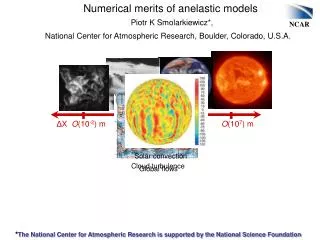
Numerical merits of anelastic models ΔXO(10-2) m O(102) m O(104) m O(107) m Gravity waves Solar convection Global flows Cloud turbulence Piotr K Smolarkiewicz*, National Center for Atmospheric Research, Boulder, Colorado, U.S.A. *The National Center for Atmospheric Research is supported by the National Science Foundation
EULAG’s key options Supported (operational in demo codes) and “private” (hidden or available in some clones) Two options for integrating fluidPDEs with nonoscillatory forward-in-time Eulerian (control-volume wise) & semi Lagrangian (trajectory wise) model algorithms, but also Adams-BashforthEulerian scheme for basic dynamics Preconditioned non-symmetric Krylov-subspace elliptic solver, but also the pre-existing MUDPACK experience. Notably, for simple problems in Cartesian geometry, the elliptic solver is direct (viz. spectral preconditioner). Generalized time-dependent curvilinear coordinates for grid adaptivity to flow features and/or complex boundaries,but also the immersed-boundary method. PDEs of fluid dynamics (comments on nonhydrostacy ~ g, xy 2D incompressible Euler): • Anelastic (incompressible Boussinesq, Ogura-Phillips, Lipps-Hemler, Bacmeister-Schoeberl, Durran) • CompressibleBoussinesq • Incompressible Euler/Navier-Stokes’ (somewhat tricky) • Fully compressible Euler/Navier-Stokes’ for high-speed flows (3 different formulations). • Boussinesq ocean model, anelastic solar MHD model, a viscoelastic ``brain’’ model, porous media model, sand dunes, dust storma, etc. Physical packages: • Moisture and precipitation (several options) and radiation • Surface boundary layer • ILES, LES, LES, DNS Analysis packages: momentum, energy, vorticitiy, turbulence and moisture budgets
Numerics related to the “geometry” of an archetype fluid PDE/ODE Eulerian conservation law Lagrangian evolution equation Kinematic or thermodynamic variables, R the associated rhs Either form is approximated to the second-order using a template algorithm:
Temporal differencing for either anelastic or compressible PDEs, depending on definitions of G and Ψ Forward in time temporal discretization Second order Taylor sum expansion about =nΔt Compensating first error term on the rhs is a responsibility of an FT advection scheme (e.g. MPDATA). The second error term depends on the implementation of an FT scheme
explicit/implicit rhs On grids co-locatedwith respect to all prognostic variables, it can be inverted algebraically toproduce an elliptic equation for pressure solenoidal velocity contravariant velocity Imposedon subject to the integrability condition Boundary conditions on Boundary value problemis solved using nonsymmetric Krylov subspace solver - a preconditioned generalized conjugate residual GCR(k) algorithm(Smolarkiewicz and Margolin, 1994; Smolarkiewicz et al., 2004) implicit: all forcings are assumed to beunknown at n+1 system implicit with respect to all dependent variables.
implicit, ~7.5 minutes of CPU explicit, ~150 minutes of CPU
Other examples include moist, Durran and compressible Euler equations. Designing principles are always the same:
Dynamic grid adaptivity Prusa & Sm., JCP 2003; Wedi & Sm., JCP 2004, Sm. & Prusa, IJNMF 2005 • A generalized mathematical framework for the implementation of deformable coordinates in a generic Eulerian/semi-Lagrangian format of nonoscillatory-forward-in-time (NFT) schemes • Technical apparatus of the Riemannian Geometry must be applied judiciously, in order to arrive at an effective numerical model. Diffeomorphic mapping (t,x,y,z) does not have to be Cartesian! Example: Continuous global mesh transformation
Example of free surface in anelastic model (Wedi & Sm., JCP,2004)
Example of IMB (Urban PBL, Smolarkiewicz et al. 2007, JCP) contours in cross section at z=10 m normalized profiles at a location in the wake
Toroidal component of B in the uppermost portion of the stable layer underlying the convective envelope at r/R≈0 .7