Turbulence Modelling: Large Eddy Simulation
Turbulence Modelling: Large Eddy Simulation. Turbulence Modeling: Large Eddy Simulation and Hybrid RANS/LES. Introduction LES Sub-grid Models Numerical aspect and Mesh Boundary conditions Hybrid approaches Sample Results. Turbulence Structures.


Turbulence Modelling: Large Eddy Simulation
E N D
Presentation Transcript
Turbulence Modeling: Large Eddy Simulation and Hybrid RANS/LES • Introduction • LES Sub-grid Models • Numerical aspect and Mesh • Boundary conditions • Hybrid approaches • Sample Results
Introduction: LES / other Prediction Methods • Different approaches to make turbulence computationally tractable: • DNS: Direct Simulation. • RANS: Reynolds average (or time or ensemble) • LES: Spatially average (or filter) • LES • 3D, unsteady DNS 3D, unsteady RANS Steady / unsteady
RANSmodel 2 LES RANS model1 RANS vs LES
Why LES? • Some applications need explicit computation of accurate unsteady fields. • Bluff body aerodynamics • Aerodynamically generated noise (sound) • Fluid-structure interaction • Mixing • Combustion • …
LES : difficulties • Cpu expensive for atmospheric modelling: • Unsteady simulation • Turn around time is weeks/months (rans is hours or days) • Cannot afford grid independence testing • Still open research issues • combustion, acoustics, high Prandtl, shmidt mixing problem, uns. • Wall bounded flows • Need expertise to reduce cpu, human cost • Mesh – models – strategy • Analysis of the instantaneous flow • Knowledge about turbulent instabilities, turbulent structures
Energy Spectrum e Eu,ET k,f • Large eddies: responsible for the transports of momentum, energy, and other scalars. anisotropic, subjected to history effects, are strongly dependent on boundary conditions, which makes their modeling difficult. Small eddies tend to be more isotropic and less flow-dependent (universal), mainly dissipative scales, which makes their modeling easier.
LES: Filtering - Decomposition Energy spectrum against the length scale Isotropic Homogeneous Universal Anisotropic Flow dependent
Filtering • The large or resolved scale field is a local average of the complete field. • e.g., in 1-D, • Where G(x,x’) is the filter kernel. • Exemple: “box filter” G(x,x’) = 1/D if |x-x’|<D/2, 0 otherwise
Filtered Navier-Stokes Equations Filtering the original Navier-Stokes equations gives filtered Navier-Stokes equations that are the governing equations in LES. N-S equation Filter Filtered N-S equation Needs modeling Sub-grid scale (SGS) stress
Available SGS model • Subgrid stress : turbulent viscosity • Smagorinsky model (Smagorinsky, 1963) • Need ad-hoc near wall damping • Dynamic model (Germano et al., 1991) • Local adaptation of the Smagorinsky constant • Dynamic subgrid kinetic energy transport model (Kim & Menon 2001) • Robust constant calculation procedure • Physical limitation of backscatter
Hypothesis: local equilibrium of sub-grid scales Simple algebraic (0-equation) model (similar to Prandtle Mixing length model in RANS) Cs= 0.065 ~ 0.25 The major shortcoming is that there is no Cs universally applicable to different types of flow. Difficulty with transitional (laminar) flows. An ad hoc damping is needed in near-wall region. Turbulent viscosity is always positive so no possibility of backscatter. Smagorinsky’s Model with
DynamicSmagorinsky’sModel • Based on the similarity concept and Germano’s identity (Germano et al., 1991; Lilly, 1992) • Introduce a second filter, called the test filter with scale larger than the grid filter scale • The model parameter (Cs ) is automatically adjusted using the resolved velocity field. • Overcomes the shortcomings of the Smagorinsky’s model. • Can handle transitional flows • The near-wall (damping) effects are accounted for. • Potential Instabilityof the constant
Dynamic Smagorinsky’s Model • Basic Idea : consider the same smagorinsky model at two different scales, and adjust the constant accordingly • Constant value = error minimization using least square method and Germano’s Identity Test Filter Grid Filter Tij Error minimization ij Lij
Dynamic Subgrid KE Transport Model • Kim and Menon (1997) • One-equation (for SGS kinetic energy) model • Like the dynamic Smagorinsky’s model, the model constants (Ck, Ce) are automatically adjusted on-the-fly using the resolved velocity field. • Backscatter better accounted for
Mesh Energie E(k) Dissipation D(k) • Grid resolution : • Constraint Based on LES hypothesis: • Explicit Resolution of production mechanism (whereas production is modeled with RANS) • Resolution of anisotropic and energetic large scales • Cell size must be included inside the inertial range, in between the integral scale (L) and the Taylor micro-scale (l). • Integral scale L • Energy peaks at the integral scale. These scales must be resolved (with several grid points). • Crude Estimation of L : • Use correlation (mixing layer, jet) for L • Perform RANS calculation and compute L = k3/2 / e 1/ 1/L 1/
Mesh • Grid resolution: • Taylor micro-scale l: • Dissipation rate peaks at l. • Not necessary to resolve l but useful to define a lower bound for the cell size. • Estimation of l ~ L ReL-1/2 • ( for an homogeneous and isotropic turbulence = 151/2 L ReL-1/2) • Temporal resolution: resolve characteristic time scale associated to the cell size (ie CFL=U Dt / Dx <1). • As for the numerical scheme (minimization of numerical errors) use of hexa and high quality of mesh (very small deformations) is recommended
Numerics: time step • Dt must be of the order (or even less for acoustic purpose) of the characteristic time scale t corresponding to the smallest resolved scales. • As t~Dx/U , it correspond to approx CFL = 1 (Courant Dreidrich Levy Number) (where U is the velocity scale of the flow)
Numerics: discretization scheme • Discretization scheme in space should minimize numerical dissipation • LES is much more sensitive to numerical diffusion than RANS • 2nd Order Central Difference Scheme (CD or BCD) perform much better than high order upwind scheme for momentum • A commonly used remedy is to blend CD and FOU. • With a fixed weight (G = 0.8), this blending scheme has been found to still introduce considerable numerical diffusion • Bad idea! • Most ideally, we need a smart, solution-adaptive scheme that detects the wiggles on-the-fly and suppress them selectively.
Boundary Conditions (LES) • Near-wall resolving • Near-wall modelling • Inlet Boundary Conditions
Inlet Boundary Conditions Inlet Boundary conditions : • Laminar case: • Random noise is sufficient for transition • Turbulent case: • Precursor domain • Realistic inlet turbulence • Cpu cost – not universal • Vortex Method • Coherent structures – preserving turbulence • Need to use realistic profiles (U, k, e) – otherwise risk to force the flow Spectral synthesizer • No spatial coherence • Flexibility for inlet (profiles of full reynolds stress or k-e, constant values, correlation)
Boundary Conditions • Near Wall treatment • 1/ Near Wall Resolving • All the near–wall turbulent structures are explicitly computed down to the viscous sub-layer. • 2/ Near Wall Modeling • All the near-wall turbulent structures are explicitly computed down to a given y+ >1 • 3/ DES: • No turbulent structures are computed at all inside the entire boundary layer (all B.L. is modeled with RANS).
Boundary Conditions • 1/ Near wall resolving : explicit resolution of the boundary layer. • Motivation: separated flows, complex physics (turbulence control) • High resolution requirement due to the presence of (anisotropic) wall turbulent structures: so called streaks. • Necessary to resolved correctly these near wall production mechanisms • Boundary layer grid resolution : • y+<2 • Dx+ ~ 50-150, Dz+ ~ 15-40 • Not only wall normal constraints, but also Span-wise and stream-wise constraintsdue to the streaky structures
Boundary Conditions • Near wall modeling : • Wall function: • Schumann/Grozbach: • Instantaneous wall shear stress at walls and instantaneous tangential velocity in the wall adjacent cells are assumed to be in phase. • Log law apply for mean velocity (necessary to perform acquisition) • Werner & Wengle (6.2): • Instantaneous wall shear stress at walls and instantaneous tangential velocity in the wall adjacent cells are assumed to be in phase. • Filtered Log law (power 1/7) applied to instantaneous quantities
Hybrid LES-URANS • Near Walls: URANS 1-equation model • Core region: LES 1-equation SGS model
Hybrid LES-URANS • Navier Stokes time averaged in the near wall and filtered in the core region reads:
LES-URANS hybrid • Use 1-equation model in both LES and URANS regions LES region RANS region
LES-URANS hybrid • Problems: • LES region is supplied with bad BC from the URANS regions • The flow going from URANS to LES region has no proper time or length scale of turbulence • Solution: • Add synthesized isotropic fluctuations as the source term of the momentum equations at the LES-URANS interface.
LES of a realistic Car model exposed to Crosswind Volume mesh: Gambit & « Sizing Functions » to control both growth rate and cell size in specified box Rear box Side box
Comparision between RANS and LES-RANS hybrid model • RANS using SST model • Hybrid RANS-LES model
Conclusion • RANS/URANS is not always reliable. • LES is closer to reality than RANS/URANS. • LES is computationally very expensive. • In the absence of enough experimental data one is left with no choice but to use LES wherever feasible.