Proportional Hazards Model

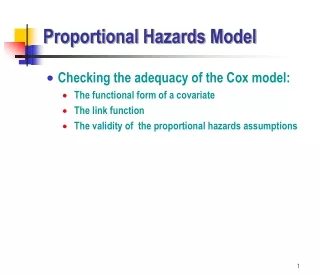
1. Proportional Hazards Model • Checking the adequacy of the Cox model: • The functional form of a covariate • The link function • The validity of the proportional hazards assumptions

2. Cox-Snell Residuals Definitions • 1. Cox-Snell Residuals • rj=-ln{S(tj ; θ̂)} • S(tj ; θ̂) is the value of the estimated survivor function at time tj. • They are just just the estimated cumulative hazard • If the model is correct, then the residuals should have an exponential distribution with mean 1. • Cox-Snell residuals are useful for assessing the fit of the parametric models • They are not very informative for Cox models estimated by partial likelihood.

3. Martingale Residuals • 2. Martingale Residuals • For a censored case, the Martingale residual is the negative of the Cox-Snell residual. For an uncensored case, it is one minus the Cox-Snell residual. • Martingale residuals can then be plotted against the respective covariate and enhance the plots by including Lowess curves (smoother) to indicate the functional form of the relationship between the log-hazard function and the covariate. • Weaknesses . They are not symmetrically distributed about zero even when the fitted model is correct . This skewness makes plots difficult to interpret.

4. Deviance Residuals Definitions • 3. Deviance Residuals • Behaving much like residuals from LS regression • Symmetrically distributed around 0 and have an approximate standard deviation of 1.0. • Are negative for observations that have longer survival times than expected and positive for observations with survival times that are smaller than expected. I • Censoring can produce striking patterns that don't necessarily imply any problem with the model itself.

5. Liver Data Example • Data data Liver; input Time Status Age Albumin Bilirubin Edema Protime @@; label Time="Follow-up Time in Years"; Time= Time / 365.25; datalines; 400 1 58.7652 2.60 14.5 1.0 12.2 4500 0 56.4463 4.14 1.1 0.0 10.6 1012 1 70.0726 3.48 1.4 0.5 12.0 1925 1 54.7406 2.54 1.8 0.5 10.3 1504 0 38.1054 3.53 3.4 0.0 10.9 2503 1 66.2587 3.98 0.8 0.0 11.0 1832 0 55.5346 4.09 1.0 0.0 9.7 2466 1 53.0568 4.00 0.3 0.0 11.0 …. ….

6. Liver Data, Fitting PH • Fitting PH Cox Model

7. Deviance Residual Diagnosis

8. Deviance Residual Diagnosis

9. Deviance Residual Diagnosis

10. Conventional Residuals Analysis Issues • highly subjective • difficult to interpret

11. New Method of Residual Diagnosis • Objective way • Checking model fit based on cumulative sumof Martingale • Asymptotic property of the sum • Gaussian Process • Bootstrapping

12. Definition of Random Process Definitions • 1. Random Process (Stochastic Process) • A random process is the counterpart to a deterministic process. • Instead of dealing with only one possible "reality" of how the process might evolve under time (as is the case, for example, for solutions of an ordinary differential equation), in a stochastic or random process there is some indeterminacy in its future evolution described by probability distributions • This means that even if the initial condition (or starting point) is known, there are many possibilities the process might go to, but some paths are more probable and others less • Example: Markov process,, Gaussian process

13. X2(t) XN(t) The totality of all sample functions is called an ensemble For a specific time X(tk) is a random variable t Definition of Random Process • Random process X(t)

14. Definition of Gaussian Process • 2. Gaussian Process A random process X(t) is a Gaussian process if for all n and for all , the random variables has a jointly Gaussian density function, which may expressed as : n random variables : mean value vector : nxn covariance matrix

15. Why Gaussian Process ? • Central limit theorem • The sum of a large number of independent and identically distributed(i.i.d) random variables getting closer to Gaussian distribution • Cumulative residuals will be centered at zero if the model is correct. • Under the null hypothesis of a correct model fit, they can be approximated as a zero mean Gaussian process with a covariance structure determined by the particular type of regression model. • Realizations of the Gaussian process can be simulated by computer and compared with the observed process to assess whether the observed residual process represents anything beyond random variation.

16. Liver Data, Residuals Diagnosis • 1. Checking the Functional Form of a Covariate

17. Liver Data, Residuals Diagnosis

18. Liver Data, Residuals Diagnosis

19. Residuals Sum Diagnosis Summary • The light dashed lines in Figure 2 are the first 20 realizations of 10,000 simulated paths of the cumulative residual process under the null hypothesis of a correct model fit. • All the paths tend to be closer to and intersect the horizontal axis compared the observed residuals. • The fitted model overestimates the hazards for the low end of the Bilirubin values and underestimate the hazards for high Bilirubin values • None of the 10,000 simulated paths has an absolute maximum exceeding that of the observed process. • Thus, the p-value for a Kolmogorov-type supremum test is 0. These results suggest that there may be a better fitting model for the surgical unit data. • The pattern suggests a logarithmic transform.

20. Fitting Cox With logBilirubin • After Fitting Cox to Liver data using logBilurubin instead of Bilirubin

21. Log Transformation of Bilirubin • Residuals Diagnosis after fitting logBilirubin

22. Comment • When the log transform is applied to Bilirubin, the observed process appears to be more typical of the simulated processes. • The p-value, based on 10,000 simulated samples, is 0.0572, indicating a much improved model

23. Checking PH Assumptions • 2. Checking Proportional Hazards Assumptions • To check the proportional hazards assumption the score process (which is a transformed partial sum process of the martingale residuals) is compared to the simulated processes under the null hypothesis that the proportional hazards assumption holds.

24. Checking PH Assumption for log(protime)

25. Comment Comment • The observed standardized score process for log(Protime) and the first 20 of 10,000 simulated null processes reveals violation of the proportional hazards assumption • As Lin et al. (1993) suggests, the violation may be corrected using time-dependent covariates or stratification

26. The Kolmogorov-type supremum test results for all the covariates • Checking PH assumption

27. Comment • In addition to log(Protime), the proportional hazards assumption appears to be violated for Edema.