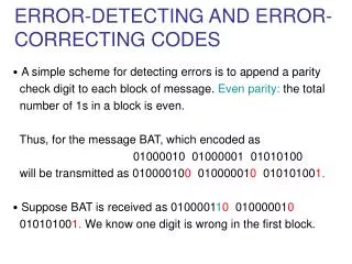
Error correcting codes
Error correcting codes. A practical problem of theoretical importance. Claude Shannon (1916-2001). 1937. MSc, MIT. 1948 – Seminal paper inventing the field of information theory.

Error correcting codes
E N D
Presentation Transcript
Error correcting codes A practical problem of theoretical importance
Claude Shannon (1916-2001) 1937. MSc, MIT. 1948 – Seminal paper inventing the field of information theory. “As a 21-year-old master's student at MIT, he wrote a thesis demonstrating that electrical application of Boolean algebra could construct and resolve any logical, numerical relationship. It has been claimed that this was the most important master's thesis of "all time.
Noisy channels • Alice wants to send Bob a binary string. • Each bit is flipped with probability p<1/2 Shannon asked: How much “information” is transferred in each bit? How many bits are needed to reliably transfer k bits of information?
Pictorially The scheme is useful if for every x, Pr[x’≠x] ε A E B Y=y1..yn Y’=y’1..y’n X {0,1}k X ‘=D(x) {0,1}k Y = E(x) {0,1}k Shannon: There exists a useful scheme (with exponentially small error) transmitting k=(1-H(p))n bits using n communication bits.
Richard Hamming(1915-1998) 1950 – motivated by the need to correct errors on magnetic storage device – defined error correcting codes. THE PURPOSE OF COMPUTING IS INSIGHT, NOT NUMBERS.
New noise model: Adversarial noise The scheme is useful if for every x, and every adversary, x’=x A E B Y=y1..yn Y’ differs in at most δ n bits from y X {0,1}k X ‘=D(x) {0,1}k Y = E(x) {0,1}k Definition: E is a (n,k,d)_ code, if E : ^k -> ^n, and for every x ≠y, d(E(x),E(y)) ≥ δn length Information bits distance Relative rate=k/n Relative distance=d/n
Rate and distance Definition: E is a (n,k,d)_ code, if E : ^k -> ^n, and for every x ≠y, d(E(x),E(y)) ≥ δn length Information bits distance Relative rate=k/n Relative distance=d/n Lemma: If E is a (n,k,d)_ code, then the encoding can detect d-1 errors and correct (d-1)/2 errors.
Linear codes Definition: Let F be a field. E is a [n,k,d]_F code, if E is a linear operator from F^k -> F^n, and for every x ≠y, d(E(x),E(y)) ≥ δn. Equivalently: C F^n is an [n,k,d]_F code if it a k-dimensional vector space over F, and has distance d. Fact: dist(C)=min_{c C} weight(c).
Gilbert-Varshamov The Gilbert Varashamov bound Proof
Stochastic vs. Adversderial noise Comparing the information rate • non-explicit lower bound • explicit lower bound • Upper bound • Current status
Algebraic-Geometric codes • Goppa
What about efficient decoding Parity-check matrix From generating matrix to parity-check matrix Testing a word Decoding Hamming codes
Decoding Reed-Solomon codes • Berlekamp • Sudan
NASA spaceships • Deep-space telecommunications • NASA has used many different error correcting codes. For missions between 1969 and 1977 the Mariner spacecraft used a Reed-Muller code. The noise these spacecraft were subject to was well approximated by a "bell-curve" (normal distribution), so the Reed-Muller codes were well suited to the situation. • The Voyager 1 & Voyager 2 spacecraft transmitted color pictures of Jupiter and Saturn in 1979 and 1980. • Color image transmission required 3 times the amount of data, so the Golay (24,12,8) code was used.[citation needed][3] • This Golay code is only 3-error correcting, but it could be transmitted at a much higher data rate. • Voyager 2 went on to Uranus and Neptune and the code was switched to a concatenated Reed-Solomon code-Convolutional code for its substantially more powerful error correcting capabilities. • Current DSN error correction is done with dedicated hardware. • For some NASA deep space craft such as those in the Voyager program, Cassini-Huygens (Saturn), New Horizons (Pluto) and Deep Space 1—the use of hardware ECC may not be feasible for the full duration of the mission. • The different kinds of deep space and orbital missions that are conducted suggest that trying to find a "one size fits all" error correction system will be an ongoing problem for some time to come.
Satellite communication Satellite broadcasting (DVB) The demand for satellite transponder bandwidth continues to grow, fueled by the desire to deliver television (including new channels and High Definition TV) and IP data. Transponder availability and bandwidth constraints have limited this growth, because transponder capacity is determined by the selected modulation scheme and Forward error correction (FEC) rate. Overview QPSK coupled with traditional Reed Solomon and Viterbi codes have been used for nearly 20 years for the delivery of digital satellite TV. Higher order modulation schemes such as 8PSK, 16QAM and 32QAM have enabled the satellite industry to increase transponder efficiency by several orders of magnitude. This increase in the information rate in a transponder comes at the expense of an increase in the carrier power to meet the threshold requirement for existing antennas. Tests conducted using the latest chipsets demonstrate that the performance achieved by using Turbo Codes may be even lower than the 0.8 dB figure assumed in early designs.
Data storage (erasure codes, systematic codes) RAID 1 RAID 1 mirrors the contents of the disks, making a form of 1:1 ratio realtime backup. The contents of each disk in the array are identical to that of every other disk in the array. A RAID 1 array requires a minimum of two drives. RAID 1 mirrors, though during the writing process copy the data identically to both drives, would not be suitable as a permanent backup solution, as RAID technology by design allows for certain failures to take place. [edit] RAID 3/4 RAID 3 or 4 (striped disks with dedicated parity) combines three or more disks in a way that protects data against loss of any one disk. Fault tolerance is achieved by adding an extra disk to the array and dedicating it to storing parity information. The storage capacity of the array is reduced by one disk. A RAID 3 or 4 array requires a minimum of three drives: two to hold striped data, and a third drive to hold parity data. [edit] RAID 5 RAID 5 (striped disks with distributed parity) combines three or more disks in a way that protects data against the loss of any one disk. It is similar to RAID 3 but the parity is not stored on one dedicated drive, instead parity information is interspersed across the drive array. The storage capacity of the array is a function of the number of drives minus the space needed to store parity. The maximum number of drives that can fail in any RAID 5 configuration without losing data is only one. Losing two drives in a RAID 5 array is referred to as a "double fault" and results in data loss. [edit] RAID 6 RAID 6 (striped disks with dual parity) combines four or more disks in a way that protects data against loss of any two disks. [edit] RAID 10 RAID 1+0 (or 10) is a mirrored data set (RAID 1) which is then striped (RAID 0), hence the "1+0" name. A RAID 1+0 array requires a minimum of four drives: two mirrored drives to hold half of the striped data, plus another two mirrored for the other half of the data. In Linux MD RAID 10 is a non-nested RAID type like RAID 1, that only requires a minimum of two drives, and may give read performance on the level of RAID 0.
Barcodes • Bernard Silver
And everywhere else Reed–Solomon codes are used in a wide variety of commercial applications, most prominently in CDs, DVDs and Blu-ray Discs, in data transmission technologies such as DSL & WiMAX, in broadcast systems such as DVB and ATSC, and in computer applications such as RAID 6 systems.
How well can we list decode RS? • S. GS • The Jhonson’s bound
Folded RS • PV • GR
Local decoding • Hadamard
Efremenko’s codes • Yachininn • Efremenko
Local testing and PCP • Irit Dinur • Ben-Sasson, Sudan,..
Randomness extractors • Trevisan
More randomness extractors • TZS • SU • U • GUV
Summary Rich theory Practical application Basic Theoretical notion – intimately related to randomness extractors/pseudo-randomness/derandomization/PCP
Many open problems • Efficient codes meeting GV? • Is the GV bound tight for binary codes? • Are the asymptotically good locally testable codes? • Efficient Local decoding with a constant number of queries? • What else can AG codes do better? (some applications in cryptography).
Implementing an AG code • Encoding • Decoding • Requires finding the relevant math packages (Macaulay2 ?)
Are AG code better than what we think? • Another look at the definition. • Implement a simple AG code (Hermitian code) And check what is its behavior relative to lower norms.