Download
1 / 52
520 likes | 708 Vues
What weakly coupled oscillators can tell us about networks and cells. Boris Gutkin Theoretical Neuroscience Group, DEC, ENS; College de France. Game Plan. Overview of mathematical framework: weakly coupled oscillators, phase models, coupling functions, phase response curves

E N D
What weakly coupled oscillators can tell us about networks and cells Boris Gutkin Theoretical Neuroscience Group, DEC, ENS; College de France
Game Plan • Overview of mathematical framework: weakly coupled oscillators, phase models, coupling functions, phase response curves • Shunting inhibition and synchrony in pairs of neurons • Adaptation and synchrony: effects of cholinergic modulation • Dendrites and oscillations: neuron as a network
Game Plan • Overview of mathematical framework: weakly coupled oscillators, phase models, coupling functions, phase response curves • Shunting inhibition and synchrony in pairs of neurons • Adaptation and synchrony: effects of cholinergic modulation • Dendrites and oscillations: neuron as a network
How to compute H? By averaging, or equivalently (Kopell & Ermentrout ‘91) by formal method due to Kuramoto (‘82): Consider 2 weakly coupled oscillators 2.1 2.6 Let uncoupled oscillators have a stable limit cycle with period T: Where X* is the solution to the linearised adjoint Then solution can be described by: 2.7 2.2 For two coupled neurons, the coupling is synaptic: G(Vpre,V)=spre(t)(Es-V) Letting We get: 2.3 2.8 Phase locked solutions when Where If 2.4 2.9 So the phase locked solution f is stable when (Hansel et al. 1995) 2.5
How to compute H? By averaging, or equivalently (Kopell & Ermentrout ‘91) by formal method due to Kuramoto (‘82): Consider 2 weakly coupled oscillators 2.1 2.6 Let uncoupled oscillators have a stable limit cycle with period T: Where X* is the solution to the linearised adjoint Then solution can be described by: 2.7 2.2 For two coupled neurons, the coupling is synaptic: G(Vpre,V)=spre(t)(Es-V) Letting We get: 2.3 2.8 Phase locked solutions when Where If 2.4 2.9 So the phase locked solution f is stable when (Hansel et al. 1995) 2.5
How to compute H? By averaging, or equivalently (Kopell & Ermentrout ‘91) by formal method due to Kuramoto (‘82): Consider 2 weakly coupled oscillators 2.1 2.6 Let uncoupled oscillators have a stable limit cycle with period T: Where X* is the solution to the linearised adjoint Then solution can be described by: 2.7 2.2 For two coupled neurons, the coupling is synaptic: G(Vpre,V)=spre(t)(Es-V) Letting We get: 2.3 2.8 Phase locked solutions when Where If 2.4 2.9 So the phase locked solution f is stable when (Hansel et al. 1995) 2.5
How to compute H? By averaging, or equivalently (Kopell & Ermentrout ‘91) by formal method due to Kuramoto (‘82): Consider 2 weakly coupled oscillators 2.1 2.6 Let uncoupled oscillators have a stable limit cycle with period T: Where X* is the solution to the linearised adjoint Then solution can be described by: 2.7 2.2 For two coupled neurons, the coupling is synaptic: G(Vpre,V)=spre(t)(Es-V) Letting We get: 2.3 2.8 Phase locked solutions when Where If 2.4 2.9 So the phase locked solution f is stable when (Hansel et al. 1995) 2.5
How to compute H? By averaging, or equivalently (Kopell & Ermentrout ‘91) by formal method due to Kuramoto (‘82): Consider 2 weakly coupled oscillators 2.1 2.6 Let uncoupled oscillators have a stable limit cycle with period T: Where X* is the solution to the linearised adjoint Then solution can be described by: 2.7 2.2 For two coupled neurons, the coupling is synaptic: G(Vpre,V)=spre(t)(Es-V) Letting We get: 2.3 2.8 Phase locked solutions when Where If 2.4 2.9 So the phase locked solution f is stable when (Hansel et al. 1995) 2.5
How to compute H? By averaging, (Kopell & Ermentrout ‘91)or by formal method due to Kuramoto (‘82): Consider 2 weakly coupled oscillators 2.1 2.6 Let uncoupled oscillators have a stable limit cycle with period T: Where X* is the solution to the linearised adjoint Then solution can be described by: 2.7 2.2 For two coupled neurons, the coupling is synaptic: G(Vpre,V)=spre(t)(Es-V) Letting We get: 2.3 2.8 Phase locked solutions when Where If 2.4 2.9 So the phase locked solution f is stable when (Hansel et al. 1995) 2.5
How to compute H? By averaging, (Kopell & Ermentrout ‘91)or by formal method due to Kuramoto (‘82): Consider 2 weakly coupled oscillators 2.1 2.6 Let uncoupled oscillators have a stable limit cycle with period T: Where X* is the solution to the linearised adjoint Then solution can be described by: 2.7 2.2 For two coupled neurons, the coupling is synaptic: G(Vpre,V)=spre(t)(Es-V) Letting We get: 2.3 2.8 Phase locked solutions when Where If 2.4 2.9 So the phase locked solution f is stable when (Hansel et al. 1995) 2.5
Type I Type II Hodd Phase Response Curve
Game Plan • Overview of mathematical framework: weakly coupled oscillators, phase models, coupling functions, phase response curves • Shunting inhibition and synchrony in pairs of neurons • Adaptation and synchrony: effects of cholinergic modulation • Dendrites and oscillations: neuron as a network Jeong and Gutkin, Neural Comp 2007
Synchrony with hyperpolarizing inhibition depolarizing hyperpolarizing stable Phase difference unstable Synaptic speed Synaptic speed Van Vreeswijk, Abbott, Ermentrout 1994
Phase Locking with Shunting Inhibition Type I Type II
Phase Locking with Shunting Inhibition Type I Type II
Key - where is Esyn wrt minimal voltage Direct simulations confirm analysis Esyn=-60 Esyn=-96
GABA is depolarising GABA is shunting GABA is hyperpolarizing Type II Type I Asynch Synchrony Bistable Asynch Synchrony Asynch
Shunting Inhibition/Excitability • Type I • Low firing rate and fast depolarizing GABA leads to in-phase synchronization for Type I oscillators. • Only the anti-phase locked solution is stable in the shunting region. • Hyperpolarizing GABAergic synapses cause the phase dynamics to • have two stable solutions. • Type II • Asynchrony with hyperpolarizing GABA • Synchrony with depolarising GABA • Bistable regime for shunting GABA -- possible appearance of clusters • Key: how is the reversal potential related to the voltage trajectory of the neuron
Game Plan • Overview of mathematical framework: weakly coupled oscillators, phase models, coupling functions, phase response curves • Shunting inhibition and synchrony in pairs of neurons • Adaptation and synchrony: effects of cholinergic modulation • Dendrites and oscillations: neuron as a network Ermentrout, Pascal, Gutkin, Neural Comp 2002 Stiefel, Gutkin, Sejnowski (in prep)
Spike Frequency Adaptation changes type I to type II dynamics when the I-K slow is voltage dependent (low threshold). Adaptation increasing Ermentrout, Pascal, Gutkin 2001
Spike Frequency adaptation changes the shape of the PRC Adaptation increasing
Blocking M-current with Cholinergic agonist changes PRC shape!
Complex interactions between adaptation currents Blocking I-M converts type II to type I Blocking I-AHP uncovers type II
I-AHP and I-M have different sensitivity to Acetylcholine I-AHP; I-M I-AHP; I-M
Game Plan • Overview of mathematical framework: weakly coupled oscillators, phase models, coupling functions, phase response curves • Shunting inhibition and synchrony in pairs of neurons • Adaptation and synchrony: effects of cholinergic modulation • Dendrites and oscillations: neuron as a network Remme, Lengyel, Gutkin (in prep)
Hot spot --- Unexciting cable -- Hot spot • If the electrotonic distance is large -- weak interactions • Can view the dendritic tree as a network of weakly coupled oscillators Intrinsic Oscillations in Dendritic Trees Michiel Remme, GNT; Mate Lengyel, Cambridge
Dynamics of dendritic oscillators Example: Morris-Lecar oscillators • Morris-Lecar (Type II) oscillators coupled via passive cable
Hodd Influence of GABA reversal Ho Young Jeong, Gatsby, UCL Hodd and Bifurcation diagram for 40 Hz Traub neuron DC injection to get 40 Hz w/o coupling synapses with time scales compatible with fast GABA
No adaptation (40Hz) No adaptation (10Hz) Adaptation (10Hz) Influence of Adaptation & Firing rate • Low firing rate can lead to in-phase synchronization but adaptation has much • stronger effect. • - The system could be bistable in the region of hyperpolarization but the shunting effect • tends to have the stable anti-phase locked solution.
Direct simulations confirm analysis: splay state 5 coupled neurons (Esyn= -20mV, b=0.1)
Type II regime Bifurcation Diagram PRC
Stability diagram for type II neurons as a function of GABA reversal
Extension to Large Network Populations of globally coupled oscillators Order parameters • Order parameters Z characterize the collective behavior of the N-neurons • - The instantaneous degree of collective behaviors can be described by the square modulus • of Z: • Synchronous state : R1 & R2 -> 1 Asynchronous state : R1 & R2 -> 0 • Two equal size cluster: R1 ->0 & R2->1 • H is the interaction function defined from two oscillator phase dynamics • - H can be approximated by using the Fourier expansion because it is the T-periodic function • This approximated function ( ) used for • simulations
Extension to Large Network H function Order parameters Rastergram Depolarizing GABA with Adaptation sync Hyperpolarizing GABA with Adaptation async Hyperpolarizing GABA without Adaptation 2-cluster 100 globally coupled phase models
PRCs from the canonical model with adaptation With adaptation subHopf Without adaptation SNIC
The Phase Model Approach • Suppose that we couple two oscillators Where G is a coupling function. • They can be changed into a phase model using the averaging method. Where H is a T-periodic interaction function.- The phase difference is introduced to see the stability of the phase-locked solutions.- When , the phase-locked solution is stable. • For membrane models,