Download
1 / 46
530 likes | 880 Vues
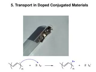
5. Transport in Doped Conjugated Materials. Nobel Prize in Chemistry 2000 . “For the Discovery and Development of Conductive Polymers”. Hideki Shirakawa University of Tsukuba. Alan MacDiarmid University of Pennsylvania. Alan Heeger University of California

E N D
Nobel Prize in Chemistry 2000 “For the Discovery and Development of Conductive Polymers” Hideki Shirakawa University of Tsukuba Alan MacDiarmid University of Pennsylvania Alan Heeger University of California at Santa Barbara
5.1. Electron-Phonon Coupling Excitations Charges E E Lowest excitation state +1 Relaxation effects Relaxation effects Absorption Ionization Emission Ground state GS Q Q Charge Transport Optical processes
5.1.1. Geometry Relaxation 14 13 15 g c a b d e f 12 16 a b c d e f g AM1(CI) Polaron / Radical-ion Polaron-exciton
5.1.2. Geometrical structure vs. Doping level Radical-cation / Polaron + Dication / Bipolaron ++
5.1.3. Geometrical Structure vs. Electronic structure E B A Bond length alternation r Within Koopmans approximation
5.1.4 Electrochromism E Neutral Bipolaron Polaron L Allowed optical transition H Spin =0 Charge = 0 Spin =1/2 Charge = +1 Spin =0 Charge = +2 Depending on the polymer and doping level, new optical transitions are possible Infra-red visible Doubly charged Neutral Singly charged
salt counterion Green-blue red
5.2. Electrochemical doping 5.2.1 Prerequisite: Reduction and oxidation reactions A reduction of a material is the gain of electrons. M + e- M- Oxy + e- Red An oxidation of a material is the loss of electrons. M M+ + e- Red Oxy + e- This system comes from the observation that materials combine with oxygen in varying amounts. For instance, an iron bar oxidizes (combines with oxygen) to become rust. We say that the iron has oxidized. The iron has gone from an oxidation state of zero to (usually) either iron II or iron III. Someone, in a fit of perversity, decided that we needed more description for the process. A material that becomes oxidized is a reducing agent (Red), and a material that becomes reduced is an oxidizing agent (Oxy).
Redox reaction is an electron transfer reaction. Since the number of electrons is constant in a system, there is no reduction of a molecule without oxidation of another chemical species. e.g.: 2Fe3+ + Sn2+ 2Fe2+ + Sn4+ Sometimes it is easier to see the transfer of electrons in the system if it is split into definite steps. Sn2+ Sn4+ + 2e- (oxidation) (2+) = (4+) + (2-) 2Fe3+ + 2e- 2Fe2+ (reduction) (6+) + (2-) = (4+) (balanced for charges) Add the two half equations: 2Fe3+ + 2e- + Sn2+ -> 2Fe2+ + Sn4+ + 2e-The electrons cancel each other out, so equation is: 2Fe3+ + Sn2+ -> 2Fe2+ + Sn4+ Fe3+ pumps the electrons from Sn2+, Fe3+ is the oxidizing agent since it helps to oxidize Sn2+.
5.2.2. One-Electron Structure Vacuum level =0 eV E EA Conduction LUMO Band IP Forbidden Band Valence HOMO Band n IP=ionization potential EA= electron affinity
Ionization potential vs. chain length n=2 n=3 n=4 n=∞ n=1 monomer n= small oligomer n= large polymer NDB = number of bonds in the conjugated pathway It is easier to remove an electron from a long oligomer (oxidize) than the monomer it-self W. Osikowicz et al., J. Chem. Phys., 119, 10415 (2003).
Conjugated polymers have a conjugated π-system and π-bands: As a result, they have a low ionization potential (usually lower than ~6eV) And/or a high electron affinity (lower that ~2eV) They will be easily oxidized by electron accepting molecules (I2, AsF5, SbF5,…) and/or easily reduced by electron donors (alkali metals: Li, Na, K) Charge transfer between the polymer chain and dopant molecules is easy When doping neutral conjugated molecules: A n-doping corresponds to a reduction (addition of electron) A p-doping corresponds to an oxidation (removal of electron)
5.2.3 Cyclic-voltammetry A. Measure the current for a linear increase of potential E (SHE) = -4.44 eV vs. Vacuum level (0 eV)
B. In electrochemical doping, the doping charge comes from an electrode. Polarons produced at potential E1 Insertion of the anions in the film + A- B+ A- Electrode B+ Electrode B+ A- A- B+ Migration of the cations In the solvent Electron transfer= positive doping E1
C. Measure the current for a cyclic linear increase of potential V Slope= scan speed time E2 0 E1 This defines the reversibility of the electrochemical reaction
D. Oxidation and Reduction When the electrode potential (V) is varied over a wide potential range, several current peak can be observed. If V> Eox, the electrode captures an electron from the organic molecule (or injection a hole). This is an oxidation or p-doping. Eox is connected to the ionization potential (IP) of the molecule. The negative counterion (anion) comes from the solution to neutralize it. If V< Ered, the electrode injects an electron. This is a reduction or n-doping. The positive counterion (cation) comes close to the negative polaron to stabilize it. Ered is related to the electron affinity (EA) oxidation reduction e EA IP LUMO e HOMO HOMO Ered Eox
A series of aromatic hydrocarbons Electronegativity EN is almost constant vs. size and close to the workfunction of graphite (4.3 eV) EN=½(IP+EA) Data taken from E. S. Chen et al, J. Chem. Phys. 110, 9310 (1999)
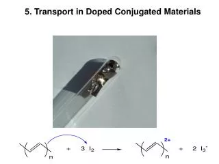
5.2.4 Electrochemical doping A. Positive doping in Poly(p-phenylenevinylene) (PPV) Radical-cation / Polaron + Dication / Bipolaron ++
Polarons produced at potential E1 Insertion of the anions in the film + A- B+ A- Electrode B+ Electrode B+ A- A- B+ Migration of the cations In the solvent Electron transfer= positive doping E1 Bipolarons produced at potential E2 A- A- ++ B+ A- A- ++ A- Electrode Electrode B+ A- A- B+ B+ A- A- Electron transfer= positive doping E2 Yes, but E1>E2 or E2>E1? Do we form directly bipolarons or first polarons then bipolarons?
B. Negative doping in poly(p-phenylene) (PPP) In electrochemical doping, a bipolaron should be formed a lower potential
C. Prove of the bipolaron hypothesis in PPP Negative doping of sexiphenyl a 2- b 3- c b c a 4- The first step (a) is a 2electron-step, thus bipolarons are formed first. No polaron is formed. Note that peaks are purely faradic, i.e., involved in an effective electron transfer
5.3. Chemical doping Electrochemical doping: the doping charge comes from the electrode and this is the ions of the salt included in the electrochemical bath that plays the role of the counterion (see previous section). Chemical doping: the doping charge (electron or hole) on the conjugated molecules or polymers comes from another chemical species C (atom or molecule). The chemical species C become the counterions of the polarons created on the conjugated materials. A strong electron donor (reducing agent) can be used to dope negatively a neutral conjugated material or to undope a positively doped material (see next slide). Example:tetrakis(dimethylamino)ethylene (TDAE), alkali metal (Li, Na, K,...) A strong electron acceptor (oxidizing agent) can be used to dope positively a neutral conjugated material or to undope a negatively doped material. Example: NOBF4 , halogen gas (I2, ...)
5.3.1 Examples of dedoping and doping DEDOPING: PEDOT-PSS (p-doped) is exposed to a vapor of TDAE and undergoes dedoping. Peaks in the IR dissapear, peak in the visible appears. The conductivity drops. PEDOT2+PS(S-)2 + TDAE→ PEDOT+TDAE+PS(S-)2 bipolarons polarons PEDOT2+PS(S-)2 + TDAE→ PEDOT+TDAE+PS(S-)2 neutral polarons DOPING: PEDOT-C14 (neutral) is exposed to a NOBF4 and undergoes doping. A first Peak in the IR appear (800-1000nm=polaron), then a second broad band at higher l. The peak in the visible disappears. The conductivity increases. PEDOT-C14 + NOBF4 → [PEDOT-C14]+BF4- + NOg neutral polarons [PEDOT-C14]+BF4- + NOBF4 →[PEDOT-C14]2+(BF4-)2+ NOg polarons K. Jeuris et al., Synth. Met. 132 (2003) 289 bipolarons F. L. E. Jakobsson et. al., Chem. Phys. Lett, 433, 110 (2006)
Doping-induced change of carrier mobilities in poly(3-hexylthiophene) films with different stacking structures. Jiang, X et. al. Chemical Physics Letters 2002, 364, (5-6), 616.
5.3.2 A special case for chemical doping: protonation of polyaniline (PAni) EB ES Emeraldine base Emeraldine salt The doping of PAni is done by protonation (using an acid), while with the other conjugated polymer it is achieved by electron transfer with a dopant or electrochemically
5.3.3. Secondary doping: Morphology change induced by an inert molecule CSA-= camphor sulfonate Example 1: polyaniline Cl-= Chlorine anion The morphology of polyaniline films is modified with the chemical nature of the acid used for doping. The doping level is not changed, but this is the nature of the counterions that induces a change in morphology and packing of the conjugated chains. CSA-, more bulky than Cl- helps the chains to pack better, such that the disorder is reduced. M. Reghu et al. PRB, 1993, 47, 1758
Example 2: Poly(3,4-Ethylenedioxythiophene) - Polystyrenesulfonate The conductivity of PEDOT-PSS increases by three orders of magnitude by using the secondary dopant diethylene glycol (DEG). This phenomena is attributed to a phase segregation of the excess PSS resulting in the formation of a three-dimensional conducting network. diethyleneglycol 100 10 1 0.1 0.01 0.001 PSS PEDOT PEDOT-PSS PSS 0.01 0.1 1 10 Conductivity (S/cm) AFM phase image %w (DEG) X. Crispin et al. Chemistry of Materials, 18, 4354 (2006) Poly(3,4-Ethylenedioxythiophene) - Polystyrenesulfonate
5.4. Variable range hopping conduction The energy difference between filled and empty states is related to the activation energy necessary for an electron hop between two sites empty states Occupied states Band edge Valence Band The charge transport occurs in a narrow energy region around the Fermi level. The charge can hop from a localized occupied state to a localized empty state that are homogeneously distributed in space and around εf. i.e. with a constant density of states N(ε) over the range [εf – ε0, εf – ε0]. N(ε)dε= number of states per unit volume in the energy range dε. 2ε0 is the width of the “band” involved in the transport. The localized character of a state is determined by the parameter r0.
In the VRH model, the reorganization energy is considered to be negligible. Hence, by assuming that, the hopping rate in the VRH becomes very similar to that used in the semi-classical electron transfer theory by Marcus. The hopping rate of the charge carrier between two sites i and j is: E = activation energy t= transfer integral N(ε)= density of states The localization radius r0 in Mott’s theory appears to be related to the rate of fall off of t with the distance rij between the two sites i and j (see previous chapter). The hopping probability from site i to site j in the transport band formed localized states is: (1)
Narrow band made of localized states • In this “band”, the average energy barrier for a charge carrier to hop from a filled to an empty state is <Eij>=ε0. (2) • The concentration C(ε0) of states in the solid characterized by the band width 2ε0 is [N(εf) 2ε0]= number of states per volume in the band. The average distance between sites involved is <rij>= [C(ε0)]-1/3= [N(εf) 2ε0]-1/3(3) The average hopping probability between two states [inject (2) and (3) in (1)]: (4)
1) First term- electronic coupling <rij>= [N(εf) 2ε0]-1/3 If wide band, i.e. ε0 large, many states are available per volume it is easy to find a neighbor site j such that Eij<ε0 <rij> decreases, t increases and kijET increases 2) Second term-activation energy <E>=ε0 If ε0 large, the activation barrier is large and the charge transfer is difficult, kijET drops The maximum for the average hopping probability is obtained for an optimal band width:
Optimal band • (i) kET or P(ε0,T) is proportional to the mobility of the charge carrier • (ii) Conductivity σ = n|e| , with n the density of charge carrier (iii) The conductivity of the entire system is determined in order of magnitude by the optimal band (States out of the band only slightly contribute to σ). Conductivity σ (T) ÷ P(ε0max,T) Mott’s law The numerical coefficient η is not determined in this course
5.4.1. Average hopping length <r> <r> = average distance rij between states in the optimal band As T decreases, the hopping length <r> grows. Indeed, as T decreases, the hopping probability decreases, so the volume of available site must be increased in order to maximize the chance of finding a suitable transport route. However the probability ω per unit time for such large hops is small: B is a numerical factor related to N(εf) In Mott’s theory, the hopping length changes with the temperature. That’s why this model is also called ”variable range hopping”.
5.4.2. Limits of Mott’s law Mott’s theory was developed for hopping transport in highly disordered system with localized states characterized by a localization length r0. Not too small values of r0 (also related to the transfer integral t) are necessary to be in the VRH regime. If r0 is too small, i.e. if the carrier wavefunction on one site is very localized, then hopping occurs only between nearest neighbors: this is the nearest-neighbor hopping regime. The situation of high disorder, thus the homogeneous repartition of levels in space and energy, is not strictly true for polymers with their long coherence length and aggregates. However, it has some success for an intermediate doping and conductivity. A more general expression is given with d the dimensionality of the transport.
When the coulomb interaction between the electron which is hopping and the hole left behind is dominant, then the conductivity dependence is In general in the semiconducting regime: Efros- Shklovskii Where x is determined by details of the phonon-assisted hopping
The resistivity ratio: ρr= ρ(1.4K)/ ρ(300K) Conductivity increases Temperature increases 5.5. Metal-Insulator transition The temperature dependence of the resistivity of PANI-CSA is sensitive to the sample preparation conditions that gives various resistivity ratios that are typically less than 50 for PANI-CSA. ρ=1/σ Metallic regime for ρr < 3: ρ(T) approaches a finite value as T0 Critical regime for ρr= 3: ρ(T) follows power-law dependence Insulating regimeρr > 3: ρ(T) follows Mott’s law ρ(T)=aT-β (0.3<β<l) Ln ρ(T)=(T0/T)1/4
The systematic variation from the critical regime to the VRH regime as the value of ρr increases from 2.94 to 4.4 is shown in the W versus T plot. This is a classical demonstration of the role of disorder-induced localization in doped conducting polymers. Zabrodskii plot The reduced activation energy: W= -T [dlnρ(T)/dT] = -d(lnρ)/d(lnT) Metallic regime: W>0 Critical regime: W(T)= constant Insulating regime: W<0 Disorder increases C.O. Yom et al. /Synthetic Metals 75 (1995) 229-239
PEDOT e- c = 7.8 Å a = 14 Å e- 3.4 Å b = 6.8 Å K.E. Aasmundtveit et al. Synth. Met. 101, 561-564 (1999) PEDOT-Tos The arrow indicates the critical regime At low T, metal regime occurs and charge carriers are delocalized Kiebooms et al. J. Phys. Chem. B 1997, 101, 11037