Heuristic Functions for Informed Search
620 likes | 736 Vues
Explore heuristic functions in informed search methods like Greedy Search and A* Search. Learn to calculate cost estimates for algorithms and evaluate heuristics. Understand how effective branching factors impact problem solving. Discover techniques for inventing heuristic functions and their application in constraint satisfaction problems (CSPs).

Heuristic Functions for Informed Search
E N D
Presentation Transcript
Course Outline 4.2Searching with Problem-specific Knowledge Presented by: Wing Hang Cheung Paul Anh Tri Huynh Mei-Ki Maggie Yang Lu Ye CPSC 533 January 25, 2000
Chapter 4 - Informed Search Methods • 4.1 Best-First Search • 4.2 Heuristic Functions • 4.3 Memory Bounded Search • 4.4 Iterative Improvement Algorithms
4.1 Best First Search • Is just a General Search • minimum-cost nodes are expanded first • we basically choose the node that appears to be best according to the evaluation function Two basic approaches: • Expand the node closest to the goal • Expand the node on the least-cost solution path
The Algorithm Function BEST-FIRST-SEARCH(problem, EVAL-FN) returns a solution sequence Inputs: problem, a problem Eval-Fn, an evaluation function Queueing-Fu a function that orders nodes by EVAL-FN Return GENERAL-SEARCH(problem, Queueing-Fn)
Greedy Search • “ … minimize estimated cost to reach a goal” • a heuristic function calculates such cost estimates h(n) = estimated cost of the cheapest path from the state at node n to a goal state
The Code Function GREEDY-SEARCH(problem) return a solution or failure return BEST-FIRST-SEARCH(problem, h) Required that h(n) = 0 if n = goal
Straight-line distance • The straight-line distance heuristic function is a for finding route-finding problem hSLD(n) = straight-line distance between n and the goal location
B 75 140 A 99 E F 118 211 80 C G 111 97 D H I 101 A E B C h=253 h=329 h=374
A h=253 E C B F G A h = 366 h = 178 h = 193 Total distance = 253 + 178 = 431 A E F h = 253 h = 178
A h = 253 E C B A F G h =366 h=178 h=193 E I h = 253 h = 0 Total distance =253 + 178 + 0 =431 A E F I h = 253 h = 178 h = 0
B 75 140 A 99 E F 118 211 80 C G 111 97 D H I 101 Optimality A-E-F-I = 431 vs. A-E-G-H-I = 418
Completeness • Greedy Search is incomplete • Worst-case time complexity O(bm) Straight-line distance h(n) A 6 A B 5 Starting node C 7 B D 0 D C Target node
B 75 140 A 99 E F 118 211 80 C G 111 97 D H I 101 A* search f(n) = g(n) + h(n) • h = heuristic function • g = uniform-cost search
“ Since g(n) gives the path from the start node to node n, and h(n) is the estimated cost of the cheapest path from n to the goal, we have… ” f(n) = estimated cost of the cheapest solution through n
f(n) = g(n) + h(n) A f =0 + 366 = 366 A E B C f=140 + 253 =393 f = 75 +374 =449 f = 118+329 =447 f = 140+253 = 393 E C B F G A f = 220+193 = 413 f = 280+366 = 646 f =239+178 =417
f =0 + 366= 366 A f = 140 + 253 = 393 E C B f =220+193 =413 A F G E H f = 317+98 = 415 f = 300+253 = 553
f =0 + 366= 366 A f(n) = g(n) + h(n) f = 140 + 253 = 393 E C B f =220+193 =413 A F G E H f = 317+98 = 415 f = 300+253 = 553 f = 418+0 = 418 I
Remember earlier A A-E-G-H-I = 418 E G H I f = 418+0 = 418
The Algorithm function A*-SEARCH(problem) returns a solution or failure return BEST-FIRST-SEARCH(problem,g+h)
Chapter 4 - Informed Search Methods • 4.1 Best-First Search • 4.2 Heuristic Functions • 4.3 Memory Bounded Search • 4.4 Iterative Improvement Algorithms
OBJECTIVE • calculates the cost estimates of an algorithm
IMPLEMENTATION • Greedy Search • A* Search • IDA*
EXAMPLES • straight-line distance to B • 8-puzzle
EFFECTS • Quality of a given heuristic • Determined by the effective branching factor b* • A b* close to 1 is ideal • N = 1 + b* + (b*)2 + . . . + (b*)d N = # nodes d = solution depth
EXAMPLE • If A* finds a solution depth 5 using 52 nodes, then b* = 1.91 • Usual b* exhibited by a given heuristic is fairly constant over a large range of problem instances
. . . • A well-designed heuristic should have a b* close to 1. • … allowing fairly large problems to be solved
NUMERICAL EXAMPLE Fig. 4.8 Comparison of the search costs and effective branching factors for the IDA and A* algorithms with h1, h2. Data are averaged over 100 instances of the 8-puzzle, for various solution lengths.
INVENTING HEURISTIC FUNCTIONS • How ? • Depends on the restrictions of a given problem • A problem with lesser restrictions is known as • a relaxed problem
INVENTING HEURISTIC FUNCTIONS Fig. 4.7 A typical instance of the 8-puzzle.
INVENTING HEURISTIC FUNCTIONS One problem … one often fails to get one “clearly best” heuristic Given h1, h2, h3, … , hm ; none dominates any others. Which one to choose ? h(n) = max(h1(n), … ,hm(n))
INVENTING HEURISTIC FUNCTIONS Another way: • performing experiment randomly on a particular problem • gather results • decide base on the collected information
HEURISTICS FORCONSTRAINT SATISFACTION PROBLEMS (CSPs) • most-constrained-variable • least-constraining-value
EXAMPLE Fig 4.9 A map-coloring problem after the first two variables (A and B) have been selected. Which country should we color next? B A C E F D
Chapter 4 - Informed Search Methods • 4.1 Best-First Search • 4.2 Heuristic Functions • 4.3 Memory Bounded Search • 4.4 Iterative Improvement Algorithms
4.3 MEMORY BOUNDED SEARCH In this section, we investigate two algorithms that are designed to conserve memory
Memory Bounded Search 1. IDA* (Iterative Deepening A*) search - is a logical extension of ITERATIVE - DEEPENING SEARCH to use heuristic information 2. SMA* (Simplified Memory Bounded A*) search
Iterative Deepening search • Iterative Deepening is a kind of uniformed search strategy • combines the benefits of depth- first and breadth-first search • advantage - it is optimal and complete like breadth first search - modest memory requirement like depth-first search
IDA* (Iterative Deepening A*) search • turning A* search IDA* search • each iteration is a depth first search ~ use an f-cost limit rather than a depth limit • space requirement ~ worse case : b f*/ b - branching factor f* - optimal solution - smallest operator cost d - depth ~ most case : b d is a good estimate of the storage requirement • time complexity -- IDA* does not need to insert and delete nodes on a priority queue, its overhead per node can be much less than that of A*
Contour IDA* search • First, each iteration expands all nodes inside the contour for the current f-cost • peeping over to find outthe nextcontour lines • once the search inside a given contour has been complete • a new iteration is started using a new f-cost for the next contour
IDA* search Algorithm function IDA* (problem) returns a solution sequence inputs: problem, a problem local variables: f-limit, the current f-cost limit root, a node root <-MAKE-NODE(INITIAL-STATE[problem]) f-limit f-COST (root) loop do solution,f-limit DFS-CONTOUR(root,f-limit) if solution is non-null then returnsolution iff-limit = then return failure; end ---------------------------------------------------------------------------------------------------------------------------------- function DFS -CONTOUR (node, f-limit) returns a solution sequence and a new f- COST limit inputs: node, a node f-limit, the current f-COST limit local variables: next-f , the f-COST limit for the next contour, initially iff-COST [node] > f-limitthen return null, f-COST [node] if GOAL-TEST [problem] (STATE[node]} then returnnode, f-limit for each node s in SUCCESSOR (node) do solution, new-f DFS-CONTOUR (s, f-limit) ifsolution is non-null then returnsolution, f-limit next-f MIN (next-f,new-f); end return null, next-f
MEMORY BOUNDED SEARCH 1. IDA* (Iterative Deepening A*) search 2. SMA* (Simplified Memory Bounded A*) search - is similar to A* , but restricts the queue size to fit into the available memory
SMA* (Simplified Memory Bounded A*) Search • advantage to use more memory -- improve search efficiency • Can make use of all available memory to carry out the search • remember a node rather than to regenerate it when needed
SMA* search (cont.) SMA* has the following properties • SMA* will utilize whatever memory is made available to it • SMA* avoids repeated states as far as its memory allows • SMA* is complete if the available memory is sufficient to store the shallowest solution path
SMA* search (cont.) SMA* properties cont. • SMA* is optimal if enough memory is available to store the shallowest optimal solution path • when enough memory is available for the entire search tree, the search is optimally efficient
Progress of the SMA* search Label: current f-cost 12 Aim: find the lowest -cost goal node with enough memory Max Nodes = 3 A - root node D,F,I,J - goal node A 13 15 B G 25 C D 20 18 H I 24 35 E F 30 24 J K 29 ---------------------------------------------------------------------------------------------------------- 12 13 (15) A 12 A A 13 A B 15 13 G B 15 G 13 • Memorize B • memory is full • H not a goal node, mark • h to infinite • Memory is full • update (A) f-cost for the min child • expand G, drop the higher f-cost leaf (B) H (Infinite) ------------------------------------------------------------------------------------------------------------ 15 (24) A 20 (24) A 15 A 15 (15) A • Drop C and add D • B memorize C • D is a goal node and it is lowest f-cost node then terminate • How about J has a cost of 19 instead of 24 ???????? 15 B 20 (infinite) B G 15 24 B G 24 (infinite) • I is goal node , but may not be the best solution • the path through G is not so great so B is generate for the second time D • Drop G and add C • A memorize G • C is non-goal node • C mark to infinite • Drop H and add I • G memorize H • update (G) f-cost for the min child • update (A) f-cost C (Infinite) 20 I 24
SMA* search (cont.) Function SMA *(problem) returns a solution sequence inputs:problem, a problem local variables: Queue, a queue of nodes ordered by f-cost Queue Make-Queue({MAKENODE(INITIALSTATE[problem])}) loop do ifQueue is empty then return failure n deepest least-f-cost node in Queue if GOAL-TEST(n) then return success s NEXT-SUCCESSOR(n) ifs is not a goal and is at maximum depth then f(s) else f(s) MAX(f(n), g(s)+h(s)) if all ofn’s successors have been generated then update n’s f-cost and those of its ancestors if necessary if SUCCESSORS(n) all in memory then remove n from Queue if memory is full then delete shallowest, highest-f-cost node in Queue remove it from its parent’s successor list insert its parent on Queue if necessary insert s on Queue end
Chapter 4 - Informed Search Methods • 4.1 Best-First Search • 4.2 Heuristic Functions • 4.3 Memory Bounded Search • 4.4 Iterative Improvement Algorithms
ITERATIVE IMPROVEMENT ALGORITHMS For the most practical approach in which • All the information needed for a solution are contained in the state description itself • The path of reaching a solution is not important Advantage: memory save by keeping track of only the current state Two major classes: Hill-climbing (gradient descent) Simulated annealing
Only record the state and it evaluation instead of maintaining a search tree FunctionHill-Climbing(problem)returnsa solution state inputs: problem, a problem local variables: current, a node next, a mode current Make-Node(Initial-State[problem]) loop do next a highest-valued successor of current if Value[next] Value[current] then return current current next end Hill-Climbing Search
