Download
1 / 45
450 likes | 470 Vues
Explore advanced performance analytics tools and methodologies through in-depth case studies and hands-on sessions. Learn to debug and analyze code effectively with BSC tools.

E N D
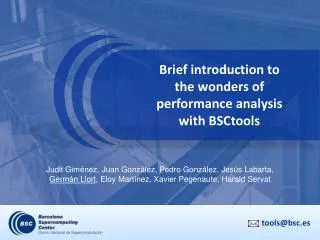
Briefintroduction to thewonders of performance analysiswithBSCtools Judit Giménez, Juan González, Pedro González, Jesús Labarta, Germán Llort, Eloy Martínez, Xavier Pegenaute, HaraldServat
Outline • Performance tools • Extrae • Paraver • Dimemas • Analysis methodology • Case study • Advanced techniques (Performance analytics) • Hands-on session
Theways of debugging & performance analysis printf(“Hellooooo!?”); … printf(“I’mhere!”); … printf(“Roger that”); gettimeofday(&start, NULL); /* Stuffthatmatters */ gettimeofday(&end, NULL); printf(“Took %d seconds to gethere”, end.tv_sec – start.tv_sec); NAS BT – 1 task A pictureisworth a thousandwords NAS BT – 32 tasks
Performance tools @ BSC Do notspeculateaboutyourcode performance LOOK AT IT Since 1991 Based on traces Flexibility and detail Core Tools Trace generation - Extrae Trace analyzer - Paraver Message passing simulator - Dimemas Open-source
Basic Workflow ROW PCF Application Process Application Process Paraver Dimemas Clustering Tracking Folding … Application Process PRV Extrae Extrae Extrae Instrumentation (Run-time) Analysis (Post-mortem)
Extrae features • Parallel programming models • MPI, OpenMP, pthreads, OmpSs, CUDA, OpenCL, Intel MIC… • Performance Counters • Using PAPI and PMAPI interfaces • Link to source code • Callstack at MPI routines • OpenMP outlined routines and their containers • Selected user functions • Periodic samples • Userevents (Extrae API) • No need to recompile / relink!
How does Extrae work? • Dynamic instrumentation • Based on DynInst (developed by U.Wisconsin/U.Maryland) • Instrumentation in memory • Binary rewriting • Symbol substitution through LD_PRELOAD • Specific libraries for each combination of runtimes • MPI • OpenMP • OpenMP+MPI • … • Alternatives • Static link (i.e., PMPI, Extrae API)
How to use Extrae? • Adapt job submission script • Tune XML configuration file • Examples distributed with Extrae • $EXTRAE_HOME/share/example • Run it! • For further reference check the Extrae User Guide: • Also distributed with Extrae at $EXTRAE_HOME/share/doc • http://www.bsc.es/computer-sciences/performance-tools/documentation
Example: Extrae with DynInst application.job #!/bin/bash … # @ total_tasks = 4 # @ cpus_per_task = 1 # @ tasks_per_node = 4 … srun./trace.sh ./my_MPI_binary #!/bin/bash … # @ total_tasks = 4 # @ cpus_per_task = 1 # @ tasks_per_node = 4 … srun ./my_MPI_binary #!/bin/sh export EXTRAE_HOME=… export EXTRAE_CONFIG_FILE=extrae.xml source ${EXTRAE_HOME}/etc/extrae.sh # Run the desired program ${EXTRAE_HOME}/bin/extrae –v $* trace.sh
Example: Extrae with LD_PRELOAD application.job #!/bin/bash … # @ total_tasks = 4 # @ cpus_per_task = 1 # @ tasks_per_node = 4 … srun ./trace.sh ./my_MPI_binary #!/bin/sh export EXTRAE_HOME=… export EXTRAE_CONFIG_FILE=extrae.xml export LD_PRELOAD=${EXTRAE_HOME}/lib/libmpitrace.so # Run the desired program $* trace.sh
LD_PRELOAD library selection 1include suffix “f” in Fortran codes Choose depending on the application type
Multiple views of the same reality Zoom in & out Apply filters to the data Highlight different aspects
Paraver displays ROW Raw time-stamped performance data MPI calls, OpenMP regions, user functions, peer-to-peer & collective communications, performance counters, samples… PCF PRV Timelines 2D / 3D Tables (statistics) 15
Timelines: Description Objects Process dimension - Thread (default) - Process - Application - Workload Resource dimension - CPU - Node - System Time
Timelines: Semantics 0 Min Max • Each window computes a function of time per object • Two types of functions • Categorical • State, user function, MPI call… • Color encoding • 1 color per value • Numerical • IPC, instructions, cache misses, computation duration… • Gradient encoding • Black(or background) for zero • From lightgreen todark blue • Limits in yellow and orange • Function line encoding
Fromtimelines to tables MPI calls profile MPI calls Computationduration Computationdurationhistogram
IPC Useful Duration L2 miss ratio Instructions Analyzing variability through histograms and timelines
Analyzing variability through histograms and timelines Useful Duration IPC Instructions L2 miss ratio By the way: six months later…
Tables: back to timelines • Where in the timeline do certain values appear? • e.g. which is the time distribution of a given routine? • e.g. when does a routine occur in the timeline?
Configuration files MPI calls profile Useful Duration Instructions executed Instructions histogram IPC User functions L2 miss ratio L2 miss ratio histogram Instructions committed Cycles wasted per L2 miss IPC histogram MPI calls Comm. bandwidth • CFG’s are programmable Paraver windows • Codify your formula once, use it forever! • Find many pre-built configurations at $PARAVER_HOME/cfgs • General • Basic views (timelines), tables(2/3D profiles), links to source code • Counters_PAPI • Hardware counter derived metrics. • Program: related to algorithmic/compilation (instructions, floating-point ops…) • Architecture: related to execution on specific architectures (cache misses…) • Performance: metrics reporting rates per time (MFLOPS, MIPS, IPC…) • MPI • Calls, peer-to-peer, collectives, bandwidth… • OpenMP • Parallel functions, outlined routines, locks… • … and many more!
B L L L CPU CPU CPU Local Local Local CPU CPU CPU Memory Memory Memory CPU CPU CPU Dimemas • Coarsegrain trace drivensimulatorfor MPI codes • Doesn’tmodeldetails • Simple MPI protocols • Abstractarchitecture • Objective • Fast & simple “what-if” analyses • Modelcomponents • Non-linear • Resourceallocation time (e.g. waitingfor output links) • Linear • Resourceusagetime (e.g. transfer time)
Dimemas vs. Paraver prv2dim <input.prv> <output.dim> • Paraver trace Whathappenswhen • Actual wallclock time of events • Dimemas trace Sequence of resourcedemands • Duration of computation bursts • Type of communication, partners and bytes • Mutual feedback • Paraver traces can be convertedintoDimemas • Dimemasgenerates as output Paraver traces of thesimulated run
Alltoall Allgather + Sendrecv Allreduce Sendrecv Waitall Real run The impossible machine • Ideal network BW = , L = 0 Transfer times gone! • Unveils the intrinsic application behavior • Load balance problems? • Serialization problems? Computation GADGET 256 tasks Nehalem cluster Ideal network
256 tasks 64 tasks Impact of architectural parameters • Ideal speeding up ALLcomputations by a constant factor • The more processes, the less speedup • The network becomes critical! GADGET 128 tasks
The potential of hybrid/accelerator parallelization % Elapsed time GADGET 128 tasks Code region 93.67% 97.49% 99.11% Speedup SELECTED regions only
Performance analysis tools objective Help generate hypotheses Help validate hypotheses Qualitatively & Quantitatively
PARAVER Tutorial Introduction to Paraver & Dimemasmethodology First steps • Parallel efficiency: Time % invested on computation • Identify sources for “inefficiency”: • Load balance • Communication / synchronization • Serial efficiency: How far from peak performance? • IPC, correlate with other counters (e.g. cache misses) • Scalability: Code replication? • Total number of instructions • Behavioral structure: Variability?
Scaling Model: Parallel Efficiency • Measured with MPI call profile • η (Parallelefficiency) • “Time % doingusefulwork” • CommEff(CommunicationEfficiency) • “Time % communicating” • LB (Load balance) • “Stallswaitingforotherranks”
Scaling Model: CommunicationEfficiency • But… • … there is another type of LB! • µLB • “Stalls due to serializations” • We measure µLB using Dimemas! • Using an ideal network Transfer efficiency = 1
AVBP (CFD) – Strong scale efficiency (12 – 960) Efficiency # Cores
Identifyingiterations Time Durationof computationsbetween MPI calls MPI ranks MPI calls
Comparingdifferentcorecounts 12 ranks 384 ranks 960 ranks • Showing 5 iterations (at different time scales) • Increasing MPI times & variability
REMEMBER Real numbersfromMPI callsprofile(η, LB, Trf) & ideal networksimulation (uLB) MeasuringParallelEfficiency • Parallel Efficiency: • η Trf • Load Balance: • Serialization: • LB • Transfer: Efficiency η # Cores
Looking at thevariability 384 tasks Computations duration MPI ranks large short Instructions
Network sensitivity (Dimemasanalysis) 384 tasks Speedup (withrespect to real run) CPU ratio
Identifyingstructure (Clusteringanalysis) Instructionscompleted IPC