Download

1 / 54
540 likes | 647 Vues
Comprehensive study on European air quality mapping using interpolation and assimilation techniques, evaluating uncertainty. Presents methodologies for data mapping and merging rural/urban maps, with emphasis on supplementary data integration.

E N D
European scale AQ mapping (using interpolation and assimilation) and evaluation of its uncertainty Jan Horálek, Pavel Kurfürst Peter de Smet ETC/ACC
Task „Spatial air quality data“ under ETC/ACC Implementation plan„to provide support in general to any AQ and spatial related activity“ – e.g. providing inputs for CSI, AP Report (maps)Final outputs of the last year:ETC/ACC Technical Paper 2005/7ETC/ACC Technical Paper 2005/8„Interpolation and assimilation methods for European scale air quality assessment and mapping“, Part I. and II.· this year Task 5.3.1.2.·MNP, CHMI, NILU
1. Interpolation of air quality data Concentration in every place is assessed by measured data from surrounding stations, especially using their linear combination: where Z(si), …, Z(si) are the concentration at the surrounding stations,li are weights. Two classes of interpolation methods: - deterministic (simple, e.g. IDW) - geostatistical (utilize spatial structure of the AQ field; different types of kriging)
2. Combination of measured AQ data and different supplementary data Supplementary (e.g. dispersion model, altitude, meteorological parameters, like temperature or wind speed, latitude or longitude) data bring more complex information about the whole area.Linear regression model of measured AQ data with supplementary data + spatial interpolation of residuals whereD1(s), …, Dm(s) are supplementary parameters in point s c, a1, …, amare parameters of linear regression model computed at the basis of data in the places of AQ stations
Mapping methodology·rural and urban maps are constructed separately (different character of urban and rural air quality) · final map is created by merging them
Rural mappingLinear regression model of measured AQ data and different supplementary data + spatial interpolation of residuals by ordinary kriging where D1(s), …, Dm(s) are supplementary data in the place s,c,a1, …, amare parameters of the regression model, computed at the places of AQ measurement.
Linear regression model – AQ measurement vs. dispersion model EMEP, altitude, sunshine duration, 2003
PM10 – rural map (combination of AQ data with EMEP dispersion model, altitude and sunshine duration), 2003
PM10 – urban map (rural map + interpolation of urban increment „Delta“), 2003
Merging of rural and urban map – using population density map
PM10 - 36. highest daily value, 2003 Combined rural and urban map
PM10 - annual average, 2003Concentration map + population density
Actual maps for 2004 plus mapping of more components resp. parameters
PM10 - 36. highest daily value, 2004Combined urban and rural map
PM10 - 56. highest daily value, 2004Combined urban and rural map
NOxrural mapping For the purposes of protection of vegetations - rural background stations only used for mapping· In this stage pure interpolation only (no use of supplem. data in places with no measurements) · 82 rural background stations with NOx data in AirBase· For some countries NOx had to be computed from NO and NO2 data in AirBase (188 stations) · For 23 stations, in which NO2 is measured only, NOx was computed based on linear regression (separately for 4 geographic areas)
Ozone -AOT40 for crops, 2004„Agricultural Areas at Risk / Damage“
Ozone - AOT40 for crops, 2004„Permanent Crops at Risk / Damage“
Ozone - AOT40 for crops, 2004„Heterogeneous Agricultural Areas at Risk / Damage“
Ozon -AOT40 for forests, 2004„Broad-Leaved Forests at Risk / Damage“
Ozon - AOT40 for forests, 2004„Coniferous Forests at Risk / Damage“
Ozon - AOT40 for forests, 2004„Mixed Forests at Risk / Damage“
Using of actual meteorological instead of long-term climatic data
Using of actual meteorological data instead of long-term climatic data Under IP2005 climatic data were used (averages 1961-1990)· This year we use actual (2004) meteorological data obtained from ECWMF. Improving of results (higher coefficient of determination R2):
Using of actual meteorological data instead of long-term climatic data Major improvement in the usability of supplementary parameters – actual wind speed improves the assessment of PM10 (contrary to climatic long term wind speed)·Caused by the differences between actual and climatic wind speed.
Comparison of actual meteorological 2004and climatic 1961-1990 data
Crossvalidation analysis of interpolation error Crossvalidation: interpolation is done without one station, repeatedly for all points – stituation in places with no measurement is simulated.· Crossvalidation gives the objective measure of the quality of interpolation. · Several indicators: root-mean-square error (RMSE), mean prediction error (MPE), absolute error (MAE) where Z(si) is a value of concentration in the i-th point Ż(si) is the estimation in the i-th point using other points· MAE should be the smallest and MPE should be the nearest to zero
Crossvalidation analysis of interpolation error Crossvalidation scatterplot: measured values and interpolated values interpolated from other stations are plotted· Linear regression of these values: In ideal case would be x=y and R2=1.
Cross-validation analysis – PM10 rural, annual average, interpolation by ord. kriging (left) and cokriging (right)
Mapping of standard prediction error Possible only for geostatistic method (kriging etc.)· Contrary to crossvalidation – this error mapping has some uncertainty in itself.
AOT40 for crops (rural areas), 2004 ordinary cokriging (using altitude)
AOT40 for crops (rural areas), 2004 ordinary cokriging - Prediction Standard Error