Download
1 / 16
160 likes | 185 Vues
This study by Martin Schraner explores the impact of solar variability, greenhouse gases, ODS, volcanoes, and QBO on climate using a global climate-chemistry model. The research covers model simulations, results, and future outlook. The simulations from 1975-2000 show varying responses to changing forcing mechanisms. The model, named SOCOL, includes a general circulation model coupled to a chemistry-transport model, spectral model with horizontal truncation, and simulations for 41 chemical species with various reactions. Modifications to the model include QBO introduction, extended radiation-chemistry coupling, handling of volcanic aerosols, and representation of solar variability. Results indicate closer agreement with observations for runs incorporating changing greenhouse gases and ODS, capturing phenomena like the ozone hole and stratospheric cooling. The model shows good agreement with stratospheric water trends but underestimates ozone trends in the lower stratosphere at high latitudes. Future work includes updates to aerosol and aerosol retrieval data.

E N D
Influence of the sun variability and other natural and anthropogenic forcings on the climate with a global climate chemistry model Martin Schraner Polyproject meeting 26. October 2004
Overview • Model simulations • Preparations / Modifications of the model • Results • Outlook Martin Schraner
Aim • Analysis of the influence of different forcing mechanisms (greenhouse gases, ODS, volcanoes, sun and QBO) on ozone, temperature and dynamics during 1975-2000 with transient model simulations Martin Schraner
SOCOL model (=Solar-Climate-Ozone Links) • General circulation model MAECHAM4 coupled to chemistry-transport model MEZON • Spectral model with T30 horizontal truncation • 39 levels, from surface to 0.01 hPa • Time step for dynamics and physics: 15 min; for radiation and chemistry: 2 hours • Simulation of 41 chemical species • Reactions: 118 gas-phase, 33 photolysis and 16 heterogeneous reactions on/in sulfate aerosol • Coupling between chemistry and GCM by ozone and water vapor Martin Schraner
Simulations Transient simulations with SOCOL for 1975-2000: • CONTROL: Control Run with constant, prescribed greenhouse gases and ODS concentrations of 1975 and a mean solar constant • GG: As 1., but with annually increasing greenhouse gases (CO2, CH4, N2O) • ODS: As 1., but with varying ODS • GG+ODS: As 1., but with changing greenhouse gases and varying ODS • GG+ODS+AER: As 4., but with volcanic aerosols • GG+ODS+AER+SOL: As 5., but with varying solar forcings (varying solar constant (-> radiation), varying photolysis rates) • GG+ODS+AER+SOL+QBO: As 6., but with nudged QBO In all simulations, continuously changing SST and SI (sea ice) are prescribed. Various ensembles of experiment 7. will be calculated. Martin Schraner
Modifications of SOCOL (1):Introduction of QBO • Model cannot simulate QBO by itself (vertical resolution not fine enough), but it can be nudged • QBO nudging by Marco Giorgetta adapted to ECHAM4 and introduced into the model Martin Schraner
0.1 0.1 0.1 1 1 1 Pressure [hPa] Pressure [hPa] Pressure [hPa] 10 10 100 100 100 1000 1000 1000 Time series of mean zonal wind over equator 1976-1980 SOCOL without QBO SOCOL with QBO Observations (Canton Island, Gan/ Maledives, Singapore) 10 1976 1977 1978 1979 Martin Schraner
Modifications of SOCOL (2):Extending the coupling of radiation code with chemistry module • Before: coupling of chemistry model with radiation module only for H2O and O3 • Now: coupling also for CH4, N2O and CFCs -> 3d-concentrations calculated in the chemistry module at every time step are used in radiation part (instead of global constant concentrations) Martin Schraner
Modifications of SOCOL (3):Introduction of volcanic aerosols and solar variability • Introduction of monthly and annually changing stratospheric aerosol dataset GISS -> altitude, latitude, and time dependent stratospheric extinction coefficients (radiation part) -> altitude, latitude, and time dependent stratospheric surface densities and thus variable heterogeneous reaction rates (hydrolysis of N2O5!) • Introduction of solar variability (combination of data from Margrit Habereiter with data from Lean) -> time dependent solar constant (radiation module) -> time dependent photolysis rates (chemistry model) Martin Schraner
Time series of total ozone averaged over 65N-65S Martin Schraner
Stratospheric aerosol extinction coefficient [1/km] (550 nm) for July 1991 – Dec 1991 SAGE 2 GISS / SAGE 2 GISS Jul 91 Aug 91 Sep 91 Oct 91 Nov 91 Dec 91 Martin Schraner
0.1 0.1 0.1 0.1 0.1 0.1 1 1 1 1 1 1 Pressure [hPa] Pressure [hPa] Pressure [hPa] Pressure [hPa] Pressure [hPa] Pressure [hPa] 10 10 10 10 10 10 100 100 100 100 100 100 1000 1000 1000 1000 1000 1000 Ozone and temperature trend(trend over 1980-1997 per decade) CONTROL GG 1 GG 2 ODS GG+ODS OBSERV Latitude Latitude Martin Schraner
0.1 0.1 0.1 0.1 0.1 1 1 1 1 1 10 10 10 10 10 Pressure [hPa¨] Pressure [hPa¨] Pressure [hPa¨] Pressure [hPa¨] Pressure [hPa¨] 100 100 100 100 100 1000 1000 1000 1000 1000 Trend for water vapor for 1975-2000 CONTROL GG 1 GG 2 ODS GG+ODS Latitude Martin Schraner
Results • The obtained temperature and ozone trends for the run with changing greenhouse gases and changing ODS are closer to observations than the runs of experiment 1., 2. and 3. • The model captures well the formation of the ozone hole over the southern high-latitudes, the ozone depletion in the upper stratosphere, the stratospheric cooling and tropospheric warming. • The model simulates an increase of the stratospheric water mixing ratio of about 7%/decade in agreement with observations. • However, the model underestimates the magnitude of ozone trends in the lower stratosphere at high latitudes Martin Schraner
Outlook (1) • Introduction of new version of tropospheric aerosol data set (U. Lohmann) • Introduction of new version of SAGE 2 retrieval (stratospheric aerosol data) into the model, incl. climatology for years without volcanoes • Rerun of all simulations with updated model version (on the available PCs, all experiments can run together and take about 3 months) Martin Schraner
Outlook (2) • Analysis of simulations. Focus on the following questions: • Does the model reproduce the observed trends in stratospheric ozone, temperature, and water vapor? • Reasons for the increase of modelled water vapor. How does (dT/dt)cold point tropopauselook like? • GG reduce ozone destruction. This is understandable for the upper stratosphere (cooling by GG slows down ozone destroying reactions), but unclear for lower stratosphere (smaller ozone hole). Major warming? Dynamical effects? • Influence of GG and ODS on stratospheric temperature: ≈1:1 at the stratopause and ≈2:1 in the lower stratosphere. More exactly quantification. Can the total temperature change be linearly combined from the single components? Martin Schraner