Download
1 / 9
100 likes | 322 Vues
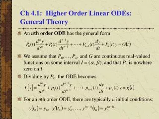
Ch 4.1: Higher Order Linear ODEs: General Theory. An n th order ODE has the general form We assume that P 0 ,…, P n , and G are continuous real-valued functions on some interval I = ( , ), and that P 0 is nowhere zero on I . Dividing by P 0 , the ODE becomes

E N D
Ch 4.1: Higher Order Linear ODEs: General Theory • An nth order ODE has the general form • We assume that P0,…, Pn, and G are continuous real-valued functions on some interval I = (, ), and that P0 is nowhere zero on I. • Dividing by P0, the ODE becomes • For an nth order ODE, there are typically n initial conditions:
Theorem 4.1.1 • Consider the nth order initial value problem • If the functions p1,…, pn, and g are continuous on an open interval I, then there exists exactly one solution y = (t) that satisfies the initial value problem. This solution exists throughout the interval I.
Example 1 • Determine an interval on which the solution is sure to exist.
Homogeneous Equations • As with 2nd order case, we begin with homogeneous ODE: • If y1,…, yn are solns to ODE, then so is linear combination • Every soln can be expressed in this form, with coefficients determined by initial conditions, iff we can solve:
Homogeneous Equations & Wronskian • The system of equations on the previous slide has a unique solution iff its determinant, or Wronskian, is nonzero at t0: • Since t0 can be any point in the interval I, the Wronskian determinant needs to be nonzero at every point in I. • As before, it turns out that the Wronskian is either zero for every point in I, or it is never zero on I.
Theorem 4.1.2 • Consider the nth order initial value problem • If the functions p1,…, pn are continuous on an open interval I, and if y1,…, yn are solutions with W(y1,…, yn)(t) 0 for at least one t in I, then every solution y of the ODE can be expressed as a linear combination of y1,…, yn:
Example 2 • Verify that the given functions are solutions of the differential equation, and determine their Wronskian.
Fundamental Solutions & Linear Independence • Consider the nth order ODE: • A set {y1,…, yn} of solutions with W(y1,…, yn) 0 on I is called a fundamental set of solutions. • Since all solutions can be expressed as a linear combination of the fundamental set of solutions, the general solution is • If y1,…, yn are fundamental solutions, then W(y1,…, yn) 0 on I. It can be shown that this is equivalent to saying that y1,…, yn are linearly independent:
Nonhomogeneous Equations • Consider the nonhomogeneous equation: • If Y1, Y2 are solns to nonhomogeneous equation, then Y1 - Y2 is a solution to the homogeneous equation: • Then there exist coefficients c1,…, cn such that • Thus the general solution to the nonhomogeneous ODE is where Y is any particular solution to nonhomogeneous ODE.