Linear Constant-coefficient Difference Equations
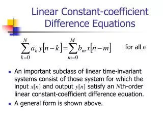
Linear Constant-coefficient Difference Equations. for all n. An important subclass of linear time-invariant systems consist of those system for which the input x [ n ] and output y [ n ] satisfy an N th-order linear constant-coefficient difference equation. A general form is shown above.

Linear Constant-coefficient Difference Equations
E N D
Presentation Transcript
Linear Constant-coefficient Difference Equations for alln • An important subclass of linear time-invariant systems consist of those system for which the input x[n] and output y[n] satisfy an Nth-order linear constant-coefficient difference equation. • A general form is shown above.
+ + + + + + + + x[n] y[n] b0 TD TD TD TD TD TD bM b2 b1 a2 aN a1 y[n-1] x[n-1] x[n-2] y[n-2] y[n-N] x[n-M] Signal Flow Graph of the Difference Equation • Assume that a0 = 1. Let TD denote one-sample delay.
Difference Equation: FIR system • The assumption a0 = 1 can be always achieved by dividing all the coefficients by a0if a00. • The difference equation characterizes a recursive way of obtaining the output y[n] from the input x[n]. • When ak = 0 for k = 1 … N, the difference equation degenerates to a FIR system. • The output consists of a linear combination of finite inputs.
Difference equation: IIR System • When bmare not all zerosfor m = 1 … M, the difference equation degenerates to • This causes an IIR system • The effect of an impulse response sequence applied to the input keeps on circulating around the feedback loops indefinitely.
Example • Accumulator
Example (continue) • Moving average system when M1=0: • The impulse response is h[n] = u[n] u[nM2 1] • Also, note that The term y[n] y[n1] suggests the implementation can be cascaded with an accumulator.
+ + + + b TD TD TD x[n] y[n] b b b x[n-1] x[n-2] x[n-M] Moving Average System • Hence, there are at least two difference equation representations of the moving average system. First, where b = 1/ (M2+1) and TD denotes one-sample delay
Moving Average System (continue) • Second, • The first representation is FIR, and the second is IIR.
Solution of Difference Equation • Just as differential equations for continuous-time systems, a linear constant-coefficient difference equation for discrete-time systems does not provide a unique solution if no additional constraints are provided. • Solution: y[n] = yp[n] + yh[n] • yh[n]: homogeneous solution obtained by setting all the inputs as zeros. • yh[n]: a particular solution satisfying the difference equation.
Solution of Difference Equation • Additional constraints: consider the N auxiliary conditions that y[-1], y[-2], …, y[-N] are given. • The other values of y[n] (n0) can be generated by when x[n] is available, y[1], y[2], … y[n], … can be computed recursively. • To generate values of y[n] for n<N recursively,
Example of the Solution • Consider the difference equation y[n] = ay[n-1] + x[n]. • Assume the input is x[n] =K [n], and the auxiliary condition is y[1] = c. • Hence, y[0] = ac+K, y[1] = a y[0]+0 = a2c+aK, … • Recursively, we found that y[n] = an+1c+anK, forn0. • For n<1, y[-2] = a1(y[1]x[1] ) = a1c, y[2] = a1 y[1] = a2 c, …, and y[n] = an+1c for n<1. • Hence, the solution is y[n] = an+1c+Kanu[n],
Example of the Solution (continue) • The recursively-implemented system for finding the solution is non-causal. • The solution system is non-linear: • When K=0, i.e., the input is zero, the solution (system response) y[n] = an+1c. • Since a linear system requires that the output be zero for all time when the input is zero for all time. • The solution system is not shift invariant: • when input were shifted by n0 samples, x1[n] =K [n - n0], the output is y1[n] = an+1c+Kann0u[n - n0].
LTI solution • Our principal interest in the text is in systems that are linear and time invariant. • How to make the recursively-implemented solution system be LTI? • Initial-rest condition: • If the input x[n] is zero for n less than some time n0, the output y[n] is also zero for n less than n0. • The previous example does not satisfy this condition since x[n]= 0 for n<0 but y[1] = c. • Property: If the initial-rest condition is satisfied, then the system will be LTI and causal.
Frequency-Domain Representation of Discrete-time Signals and Systems • Eigen function of a LTI system • When apply an eigenfunction as input, the output is the same function multiplied by a constant. • x[n] = ejwn is the eigenfunction of all LTI systems. • Let h[n] be the impulse response of an LTI system, when ejwn is applied as the input,
Eigenfunction of LTI • Let we have • consequently, ejwn is the eigenfunction of the system, and the associated eigenvalue is H(ejw). • We call H(ejw) the LTI system’s frequency response that consists of the real and imaginary parts, H(ejw)=HR(ejw)+jHI(ejw), or in terms of magnitude and phase,
Example of Frequency Response • Frequency response of the ideal delay system, y[n] =x[n nd], • If we consider x[n] = ejwn as input, then Hence, the frequency response is • The magnitude and phase are
Linear Combination • When a signal can be represented as a linear combination of complex exponentials: By the principle of superposition, the output is • Thus, we can find the output if we know the frequency response of the system.
Example of Linear Combination • Sinusoidal responses of LTI systems: • The response of x1[n] and x2[n] are • If h[n] is real, it can be shown that H(e-jw0) = H*(ejw0), the total response y[n]=y1[n]+ y2[n] is
Difference to Continuous-time System Response • For a continuous-time system, the frequency response is not necessarily to be periodic. • However, for a discrete-time system, the frequency response is always periodic with period 2, since • Because H(ejw) is periodic with period 2, we need only specify H(ejw) over an interval of length 2, eg., [0,2] or [,]. For consistency, we choose the interval [,]. • The inherent periodicity defines the frequency response everywhere outside the chosen interval.
Ideal Frequency-selective Filters • The “low frequencies” are frequencies close to zero, while the “high frequencies” are those close to . • Since that the frequencies differing by an integer multiple of 2 are indistinguishable, the “low frequency” are those that are close to an even multiple of , while the “high frequencies” are those close to an odd multiple of . • Ideal frequency-selective filters: • An important class of linear-invariant systems includes those systems for which the frequency response is unity over a certain range of frequencies and is zero at the remaining frequencies.
Frequency Response of the Moving-average System • The impulse response of the moving-average system is • Therefore, the frequency response is • By noting that the following formula holds:
Frequency Response of the Moving-average System (continue) (magnitude and phase)
Frequency Response of the Moving-average System (continue) M1= 0 and M2 = 4 Amplitude response Phase response 2w
Suddenly Applied Complex Exponential Inputs • In practice, we may not apply the complex exponential inputs ejwn to a system, but the more practical-appearing inputs of the form x[n] = ejwn u[n] • i.e., complex exponentials that are suddenly applied at an arbitrary time, which for convenience we choose n=0. • Consider its output to a causal LTI system:
Suddenly Applied Complex Exponential Inputs (continue) • We consider the output for n 0. • Hence, the output can be written as y[n] = yss[n] + yt[n], where Steady-state response Transient response
Suddenly Applied Complex Exponential Inputs (continue) • If h[n] = 0 except for 0 n M(i.e., a FIR system),then the transient response yt[n] = 0 for n+1 > M. That is, the transient response becomes zero since the time n = M. For n M, only the steady-state response exists. • For infinite-duration impulse response (i.e., IIR) • For stable system, Qn must become increasingly smaller as n , and so is the transient response.
Suddenly Applied Complex Exponential Inputs (continue) Illustration for the FIR case by convolution
Suddenly Applied Complex Exponential Inputs (continue) Illustration for the IIR case by convolution
Representation of Sequences by Fourier Transforms • Fourier Representation: representing a signal by complex exponentials. • A signal x[n] is represented as the Fourier integral of the complex exponentials in the range of frequencies [,]. • The weight X(ejw) of the frequency applied in the integral can be determined by the input signal x[n], and X(ejw) reveals how much of each frequency is required to synthesize x[n]. Inverse Fourier transform Fourier transform (or forward Fourier transform)
Representation of Sequences by Fourier Transforms (continue) • The phase X(ejw) is not uniquely specified since any integer multiple of 2 may be added to X(ejw) at any value of w without affecting the result. • Denote ARG[X(ejw)] to be the phase value in [,]. • Since the frequency response of a LTI system is the Fourier transform of the impulse response, the impulse response can be obtained from the frequency response by applying the inverse Fourier transform integral:
Existence of Fourier Transform Pairs • Whey they are transform pairs? Consider the integral
Conditions for the Existence of Fourier Transform Pairs • Conditions for the existence of Fourier transform pairs of a signal: • Absolutely summable • Mean-square convergence: In other words, the error |X(ejw) XM(ejw) | may not approach for each w, but the total “energh” in the error does.
Conditions for the Existence of Fourier Transform Pairs (continue) • Still some other cases that are neither absolutely summable nor mean-square convergence, the Fourier transform still exist: • Eg., Fourier transform of a constant, x[n] = 1 for all n, is an impulse train: • The impulse of the continuous case is a “infinite heigh, zero width, and unit area” function. If some properties are defined for the impulse function, then the Fourier transform pair involving impulses can be well defined too.
Conditions for the Existence of Fourier Transform Pairs (continue) • Properties of continuous impulse function: • Eg., consider a sequence whose Fourier transform is the periodic impulse train then the sequence is a complex exponential sequence (note that extends only over one period, from, we need include the term)
Symmetry Property of the Fourier Transform • Conjugate-symmetric sequence: xe[n] = xe*[n] • If a real sequence is conjugate symmetric, then it is called an even sequence satisfying xe[n] = xe[n]. • Conjugate-asymmetric sequence: xo[n] = xo*[n] • If a real sequence is conjugate antisymmetric, then it is called an odd sequence satisfying x0[n] = x0[n]. • Any sequence can be represented as a sum of a conjugate-symmetric and asymmetric sequences, x[n] =xe[n] + xo[n], where xe[n] = (1/2)(x[n]+ x*[n]) and xo[n] = (1/2)(x[n] x*[n]).
Symmetry Property of the Fourier Transform (continue) • Similarly, a Fourier transform can be decomposed into a sum of conjugate-symmetric and anti-symmetric parts: X(ejw) = Xe(ejw) + Xo(ejw) , where Xe(ejw) = (1/2)[X(ejw) + X*(ejw)] and Xo(ejw) = (1/2)[X(ejw) X*(ejw)]
Symmetry Property of the Fourier Transform (continue) • Fourier Transform Pairs (if x[n] X(ejw)) • x*[n] X*(e jw) • x*[n] X*(ejw) • Re{x[n]} Xe(ejw) (conjugate-symmetry part ofX(ejw)) • jIm{x[n]} Xo(ejw) (conjugate anti-symmetry part ofX(ejw)) • xe[n] (conjugate-symmetry part ofx[n]) XR(ejw) = Re{X(ejw)} • xo[n] (conjugate anti-symmetry part ofx[n]) jXI(ejw) = jIm{X(ejw)}
Symmetry Property of the Fourier Transform (continue) • Fourier Transform Pairs (if x[n] X(ejw)) • Any realxe[n] X(ejw) = X*(ejw) (Fourier transform is conjugate symmetric) • Any realxe[n] XR(ejw) = XR(ejw) (real part is even) • Any realxe[n] XI(ejw) = XI(ejw) (imaginary part is odd) • Any realxe[n] |XR(ejw)| = |XR(ejw)| (magnitude is even) • Any realxe[n] XR(ejw)= XR(ejw) (phase is odd) • xo[n] (even part of realx[n]) XR(ejw) • xo[n] (odd part of realx[n]) jXI(ejw)
Example of Symmetry Properties • The Fourier transform of the real sequence x[n] = anu[n] for a < 1 is • Its magnitude is an even function, and phase is odd.
Fourier Transform Theorems • Linearity x1[n] X1(ejw), x2[n] X2(ejw) implies that a1x1[n] + a2x2[n] a1X1(ejw) + a2X2(ejw) • Time shifting x[n] X(ejw) implies that
Fourier Transform Theorems (continue) • Frequency shifting x[n] X(ejw) implies that • Time reversal x[n] X(ejw) If the sequence is time reversed, then x[n] X(ejw) Furthermore, ifx[n] is real then x[n] X*(ejw), since X(ejw) is conjugate symmetric.
Fourier Transform Theorems (continue) • Differentiation in frequency x[n] X(ejw) implies that • Parseval’s theorem x[n] X(ejw) implies that
Fourier Transform Theorems (continue) • The convolution theorem x[n] X(ejw) and h[n] H(ejw), and ify[n] = x[n] h[n], then Y(ejw) = X(ejw)H(ejw) • The modulation or windowing theorem x[n] X(ejw) and w[n] W(ejw), and ify[n] = x[n]w[n], then a periodic convolution