Download
1 / 31
310 likes | 457 Vues
Large-Scale Molecular mapping Key Issues in Star Formation Lee Mundy (University of Maryland) a nd MSIP c loud mapping team led by John Carpenter. Credit: Herschel Gould Belt Project lead by P. Andre; Arzoumanian et al 2011. Key Issues in Star Formation.

E N D
Large-Scale Molecular mapping Key Issues in Star Formation Lee Mundy (University of Maryland) and MSIP cloud mapping team led by John Carpenter Credit: Herschel Gould Belt Project lead by P. Andre; Arzoumanian et al 2011
Key Issues in Star Formation • How do clouds evolve to the threshold of star formation? • What controls the rate of star formation in molecular clouds? • Is the stellar initial mass function imprinted in the structure of molecular clouds? Molecule line images with spatial dynamic range from 1000 AU to 10 pc will give the statistical sampling of the structure and kinematics needed to answer these questions.
Key Issues in Star Formation • How do clouds evolve to the threshold of star formation? • What controls the rate of star formation in molecular clouds? • Is the stellar initial mass function imprinted in the structure of molecular clouds? Molecule line images with spatial dynamic range from 1000 AU to 10 pc will give the statistical sampling of the structure and kinematics needed to answer these questions.
IC 5146 Star forming regionHerschel 70, 250, 500 microns color composite 30’ = 4.4 pc 500 pc away Resolution ~30” = 15,000 AU = 0.07 pc Credit: Herschel Gould Belt Project led by P. Andre; Arzoumanian et al 2011
How do clouds evolve to the threshold of star formation? Known for over 30 years, molecular clouds are largely low density: • mean volume density of 100’s particles per cc • physical density ~ 1,000 per cc in gas with CO emission The dense gas (> 104 per cc) is: • small fraction of the gas mass in the cloud but • dominates the star forming action. What mechanisms shape the structure in clouds and the formation of dense gas regions? turbulence, magnetic fields, external interactions
Herschel 250,350,500 Polaris Region of non-star formation 60 filaments with typical width of 0.1 pc 300 compact cores of which hardly any are bound Distance of 150 pc 4500 AU resolution Men’shchikov et al 2010
Numerical Simulation of hydrodynamic turbulence with modeling of atomic to molecular transition in external radiation field by Offner et al 2013 -1.0 -0.5 0.0 0.5 1.0 -1.0 -0.5 0.0 0.5 1.0 L(pc) Offner et al 2013
How do clouds evolve to the threshold of star formation? Column density PDF from simulation – isothermal, hydrodynamics with self-gravity and AMR -- Kritsuk et al. 2011 The red is the initial distribution The blue curve is a later time after the turbulence has evolved and created higher column density regions. t = 0 t = 0.43 ff log10PDF Power-law -2.5 Log-normal 0 1 2 3 Log10Σ/〈Σ〉 Hennebelle and Falgarone 2012 Kritsuk et al. (2011)
Herschel 70, 250, 500 microns Star formation region in Aquila 1 degree = 4.5 pc 700 compact condensations Estimated 100 protostars Men’shchikov et al 2010 Distance of 260 pc 7500 AU resolution Herschel Gould Belt Project led by P. Andre
How do clouds evolve to the threshold of star formation? Column density PDF for the Aquila star-forming molecular based Herschel column density images from 250, 350, 500 micron emission. Power-law Log-normal Hennebelle and Falgarone 2012 Andre et al 2011
How do clouds evolve to the threshold of star formation? The velocity field information on similar scales is needed. Magnetic fields, if dynamically significant, should show as anisotopies the velocity fields and structure. At 30” resolution, the Herschel linear resolution is limiting: 4,500 AU for closest clouds 15,000 AU for 500 pc 60,000 AU for 2 kpc CARMA observations of 12CO and 13CO can probe the gas for Av > 2 to acquire kinematics and column density structure with 5-10” resolution.
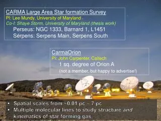
CARMA Mosaic of the Orion A Molecular Cloud Key Project started in the current semester to map 1 square degree of the Orion A Molecular Cloud in CO isotopes, CN, SO, and CS with 0.5 – 1K sensitivity in an 0.5 km/sec channel. PI: John Carpenter. Combining CARMA and Nobeyama 45-m data.
Is the stellar initial mass function imprinted in the structure of molecular clouds? A number of studies have found that the Clump Mass Function (CMF) in dense gas is related to the Initial Mass Function (IMF) for stars. CMF for starless cores in the Aquila field based on Herschel data. 452 cores identified Expect that most are bound. Konyves et al 2010
Is the stellar initial mass function imprinted in the structure of molecular clouds? However, a simple correspondence between the CMF and IMF is surprising: • “one clump”, one star? Resolution is important. • Why is there a constant fraction of the clump that goes into a star? • The turnover in the CMF typically occurs around the completeness limit. What about formation of stellar clusters where most stars form? In this environment do protostars compete for material?
Is the stellar initial mass function imprinted in the structure of molecular clouds? Krumholz et al 2011 modeled the formation of Orion type cluster in a gravitationally bound large core. Radiative feedback suppressed formation of new stars after 10-20% of the mass was in stars. Existing stars continued to feed creating a top-heavy IMF. The colored lines are for three different runs: low-resolution, high-resolution, and isothermal
Is the stellar initial mass function imprinted in the structure of molecular clouds? To understand the CMF-IMF connection, you need: • resolution to scales relevant to individual star formation -- ~1000 AU • column density and kinematic information • density information • All of above in regions covering a range of star formation activity Imaging of molecular emission gives structure and kinematics. It is critical to link structure from 1pc to ~1,000 AU scale. It is critical to use dyes to track gas at different densities.
One… and you’re NOT done Doing one molecular line is not enough. Why? Molecules trace the gas in differ ways. • 12CO: high abundance and easily excited – tracer of low density gas • 13CO and C18O: like 12CO except lower opacity so higher column density • HCN: moderate abundance high density gas tracer • HCO+: high density gas tracer bias towards regions with strong ion chemistry • H13CO+: high density gas tracer bias towards high column density • N2H+: high density gas tracer bias towards cold dense regions • CO, SO and SiO: tracers of outflow activity Good News: you can get all of these lines in two correlator settings
CARMALargeAreaStar-formationSurveY • Completing observations of 5 regions of 120-200 square arcminutes with 7” angular resolution in the J=1-0 transitions of HCO+, HCN, and N2H+ • Regions are in the Perseus and Serpens molecular clouds – covered by the c2d Spitzer Legacy project which characterized the young stellar population. • Using CARMA to get interferometric and single-dish data to make maps of the full emission.
NGC 1333 SVS -13 Region N2H+ Emission Velocity Field HCO+ Emission HCN Emission
Beam size in above three maps Provides resolution to study individual objects in the context of the large scale cloud.
NGC 1333 SVS-13 Herschel 350 microns versus N2H+ N2H+ emission tracks the structure in the long wavelength continuum…. The bright region to the northeast is a heated area associated with a reflection nebula. N2H+ traces gas >105 per cc and give velocity information.
Analyzing the Structure with Dendrograms Kirk et al 2013 Houlahan & Scalo 1992
Dendrogram of NGC 1333 • Captures the hierarchial structure • Enables analysis of kinematics and structure • Shaye Storm’s talk will cover this.
Mapping with upgraded CARMA • Dual polarization 3mm receivers • 8-band 23-element correlator Expect mapping to be ~5 times faster than current array. 8 correlator bands allow more lines to be mapped simultaneously For example: 1 square degree in the CO and CO-isotopic lines with 0.1 km/sec velocity resolution 10” angular resolution 0.5 K RMS in 10” beam
Goal: Measure the statistical structure and kinematics of large scale clouds to determine the driving scale of turbulence, the energy cascade, and the role of magnetic fields. Observation: Image 30 - 70 pc2 area of several nearby clouds in CO, 13CO, C18O with 10” resolution and 0.1 km/sec velocity resolution with CARMA and single-dish from Nobeyama 45-m Time: 300 hours per square degree to achieve 0.5 K in CO, and 0.3 K in 13CO and C18O Result: Combined with Herschel and other dust continuum images, gives the definitive dataset for large scale cloud structure CARMA Experiment #1
For example, the area of Serpens Molecular Cloud to the right is about 1.5 square degrees and covers a 7 x 10 pc region. 10” resolution corresponds to 4,000 AU 1800 pointing mosaic and 450 hours
Goal: Measure the clump mass function for a number of dense gas regions with different levels of star formation activity Observation: Image 1 x 1 pc to 2 x 2 pc area with dense gas with 3-5” resolution and 0.1 km/sec velocity resolution in the regions from Experiment #1. Combining CARMA and Nobeyama single dish data. Time: 600 hours to achieve 0.3 K over 20’ x 20’ regions with 0.1 km/sec velocity resolution in HCN, H13CN, HCO+, H13CO+, and N2H+ Result: Complete picture of structure of dense gas CARMA Experiment #2
Goal: To follow the kinematics and structure of molecular clouds from pc’s to 1,000 AU scales to show the roles of the processes that drive star formation and the nature of the stellar outcomes – over a range of star formation conditions Observations: Image 5-8 clouds at distances of 300 to 2,000 pc in CO isotopes and dense gas tracers, using the same linear resolution and Kelvin sensitivity Time requirement: 1,000-2,000 hours per cloud… roughly 8,000 hours CARMA Experiment
Herschel 70, 160, 250 W3 Massive Star Formation Region One of largest clouds in outer galaxy Spans almost 200 pc 30” = 17.5 pc Distance of 2 kpc