Wireless Systems: Modulation Schemes and Bandwidth
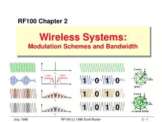
b. Q axis. f c. a. Upper Sideband. Lower Sideband. f. c. 1 0 1 0. I axis. f c. QPSK. 1 0 1 0. b. Q axis. r. a. f c. f. c. I axis. 1 0 1 0. p. v. p /4 shifted DQPSK. f c. RF100 Chapter 2. Wireless Systems: Modulation Schemes and Bandwidth.

Wireless Systems: Modulation Schemes and Bandwidth
E N D
Presentation Transcript
b Q axis fc a Upper Sideband Lower Sideband f c 1 0 1 0 I axis fc QPSK 1 0 1 0 b Q axis r a fc f c I axis 1 0 1 0 p v p/4 shifted DQPSK fc RF100 Chapter 2 Wireless Systems: Modulation Schemes and Bandwidth RF100 (c) 1998 Scott Baxter
SIGNAL CHARACTERISTICS The complete, time-varying radio signal Natural Frequency of the signal S(t)= A cos [ wc t + j] Amplitude (strength) of the signal Phase of the signal Different Amplitudes Different Frequencies Different Phases Characteristics of a Radio Signal • The purpose of telecommunications is to send information from one place to another • Our civilization exploits the transmissible nature of radio signals, using them in a sense as our “carrier pigeons” • To convey information, some characteristic of the radio signal must be altered (I.e., ‘modulated’) to represent the information • The sender and receiver must have a consistent understanding of what the variations mean to each other • “one if by land, two if by sea” • Three commonly-used RF signal characteristics which can be varied for information transmission: • Amplitude • Frequency • Phase Compare these Signals: RF100 (c) 1998 Scott Baxter
AM: Our First “Toehold” for Transmission • The early radio pioneers could only turn their crude transmitters on and off. They could form the dots and dashes of Morse code. The first successful radio experiments happened during the mid-1890’s by experimenters in Italy, England, Kentucky, and elsewhere. • By 1910, vacuum tubes gave experimenters better control over RF power generation. RF power could now be linearly modulated in step with sound vibrations. Voices and music could now be transmitted!! Still, nobody anticipated FM, PM, or digital signals. • Commercial public AM broadcasting began in the early 1920’s. • Despite its disadvantages and antiquity, AM is still alive: • AM broadcasting continues today in 540-1600 KHz. • AM modulation remains the international civil aviation standard, used by all commercial aircraft (108-132 MHz. band). • AM modulation is used for the visual portion of commercial television signals (sound portion carried by FM modulation) • Citizens Band (“CB”) radios use AM modulation • Special variations of AM featuring single or independent sidebands, with carrier suppressed or attenuated, are used for marine, commercial, military, and amateur communications SSB LSB USB RF100 (c) 1998 Scott Baxter
TIME-DOMAIN VIEW of AM MODULATOR + S a mn(t) x(t) + cos wc 1 x(t)=[1 + amn(t)]cos wct where: a = modulation index (0 < a <= 1) mn(t) = modulating waveform wc = 2p fc, the radian carrier freq. FREQUENCY-DOMAIN VIEW CARRIER mn(t) BASEBAND LOWER SIDEBAND UPPER SIDEBAND Voltage x(t) fc 0 Frequency Amplitude Modulation (“AM”) Details • AM is “linear modulation” -- the spectrum of the baseband signal translates directly into sidebands on both sides of the carrier frequency • Despite its simplicity, AM has definite drawbacks which complicate its use for wireless systems: • Only part of an AM signal’s energy actually carries information (sidebands); the rest is the carrier • The two identical sidebands waste bandwidth • AM signals can be faithfully amplified only by linear amplifiers • AM is highly vulnerable to external noise during transmission • AM requires a very high C/I (~30 to 40 dB); otherwise, interference is objectionable RF100 (c) 1998 Scott Baxter
TIME-DOMAIN VIEW: AM MODULATOR Lin. [1 + amn(t)] information Modulated signal ~ mn(t) Sat. RF carrier ~ x(t) cos wc TIME-DOMAIN VIEW: AM DETECTOR (non-coherent) mn(t) ~ x(t) Circuits to Generate & Detect AM Signals • AM modulation can be simply accomplished in a saturated amplifier • superimpose the modulating waveform on the supply voltage of the saturated amplifier • AM de-modulation (detection) can be easily performed using a simple envelope detector • example: half-wave rectifier • this “non-coherent” detection works well if S/N >10 dB. • AM demodulation can also be performed by coherent detectors • incoming signal is mixed (multiplied) with a locally generated carrier • enhances performance when S/N ratio is poor (<10 dB.) RF100 (c) 1998 Scott Baxter
TIME-DOMAIN VIEW t sFM(t)=A cos [wc t + mw m(x)dx+j0] t0 where: A = signal amplitude (constant) wc = radian carrier frequency mw = frequency deviation index m(x) = modulating signal j0 = initial phase FREQUENCY-DOMAIN VIEW LOWER SIDEBANDS UPPER SIDEBANDS SFM(t) Voltage fc 0 Frequency Better Quality: Frequency Modulation (“FM”) • Frequency Modulation (FM) is a type of angle modulation • in FM, the instantaneous frequency of the signal is varied by the modulating waveform • Advantages of FM • the amplitude is constant • simple saturated amplifiers can be used • the signal is relatively immune to external noise • the signal is relatively robust; required C/I values are typically 17-18 dB. in wireless applications • Disadvantages of FM • relatively complex detectors are required • a large number of sidebands are produced, requiring even larger bandwidth than AM RF100 (c) 1998 Scott Baxter
TIME-DOMAIN VIEW: FM MODULATOR information FM modulated signal m(x) VCO sFM(t) ~ x HPA LO TIME-DOMAIN VIEW: FM DETECTOR m(x) sFM(t) PLL x LNA LO Circuits to Generate and Detect FM Signals • One way to build an FM signal is a voltage-controlled oscillator • the modulating signal varies a reactance (varactor, etc.) or otherwise changes the frequency of the oscillator • the modulation may be performed at a low intermediate frequency, then heterodyned to a desired communications frequency • FM de-modulation (detection) can be performed by any of several types of detectors • Phase-locked loop (PLL) • Pulse shaper and integrator • Ratio Detector RF100 (c) 1998 Scott Baxter
Edwin Howard Armstrong 1890 - 1954 The Inventor of FM Major Edwin H. Armstrong was one of the most famous inventors in the early history of radio. In 1918, he invented the superheterodyne circuit -- and implemented the basic mixing principle of heterodyne frequency conversion used in virtually all modern radio receivers. Others got the credit. In 1933, he invented wide-band frequency modulation. Armstrong’s primary motivation was to improve the audio quality of broadcast transmission, which had suffered from noise and static because it used AM modulation. Promotion and commercial development of FM placed Armstrong in competition with David Sarnoff and Radio Corporation of America. Sarnoff and RCA were promoting television, and worried Armstrong’s FM would compete with TV and slow its public acceptance. Mainly due to RCA influence, the US FCC decided to change the frequencies allocated for FM broadcasting, obsoleting hundreds of FM transmitters and 500,000+ home receivers Armstrong had helped finance as an FM demonstration. In 1954, despondent over these setbacks, Armstrong took his life. But today, the technology he started is used not only in broadcasting and the sound portion of TV, but also in land mobile and first-generation analog cellular systems. RF100 (c) 1998 Scott Baxter
TIME-DOMAIN VIEW sPM(t)=A cos [wc t + mw m(x)+j0] where: A = signal amplitude (constant) wc = radian carrier frequency mw = phase deviation index m(x) = modulating signal j0 = initial phase FREQUENCY-DOMAIN VIEW LOWER SIDEBANDS UPPER SIDEBANDS SFM(t) Voltage fc 0 Frequency Sister of FM: Phase Modulation (“PM”) • Phase Modulation (PM) is a type of angle modulation, closely related to FM • the instantaneous phase of the signal is varied according to the modulating waveform • Advantages of PM: very similar to FM • the amplitude is constant • simple saturated amplifiers can be used • the signal is relatively immune to external noise • the signal is relatively robust; required C/I values are typically 17-18 dB. in wireless applications • Disadvantages of PM • relatively complex detectors are required, just like FM • a large number of sidebands are produced, just like FM, requiring even larger bandwidth than AM Phase-modulated signal information RF100 (c) 1998 Scott Baxter
TIME-DOMAIN VIEW: PHASE MODULATOR m(x) Phase Shifter sFM(t) x HPA ~ LO TIME-DOMAIN VIEW: FM DETECTOR FOR PM m(x) sFM(t) PLL x LNA LO Circuits to Generate and Detect PM Signals • PM and FM signals are identical with only one exception: in FM, the analog modulating signal is inherently de-emphasized by 1/F • Consequences of this realization: • the same types of circuitry can be used to generate and detect both analog PM or FM, determined by filtering the modulating signal at baseband • FM has poorer signal-to-noise ratio than PM at high modulating frequencies. Therefore, pre-emphasis and de-emphasis are often used in FM systems information Phase-modulated signal The phase of a PM signal is proportional to the amplitude of the modulating signal. The phase of an FM signal is proportional to the integral of the amplitude of the modulating signal. RF100 (c) 1998 Scott Baxter
Time-Domain (as viewed on an Oscilloscope) Frequency-Domain (as viewed on a Spectrum Analyzer) Voltage Voltage 0 Frequency Time fc Upper Sideband Lower Sideband fc fc fc How Much Bandwidth do Signals Occupy? • The bandwidth occupied by a signal depends on: • input information bandwidth • modulation method • Information to be transmitted, called “input” or “baseband” • bandwidth usually is small, much lower than frequency of carrier • Unmodulated carrier • the carrier itself has Zero bandwidth!! • AM-modulated carrier • Notice the upper & lower sidebands • total bandwidth = 2 x baseband • FM-modulated carrier • Many sidebands! bandwidth is a complex Bessel function • Carson’s Rule approximation 2(F+D) • PM-modulated carrier • Many sidebands! bandwidth is a complex Bessel function RF100 (c) 1998 Scott Baxter
Digital Sampling and Vocoding RF100 (c) 1998 Scott Baxter
transmission demodulation-remodulation transmission demodulation-remodulation transmission demodulation-remodulation Introduction to Digital Modulation • The modulating signals shown in previous slides were all analog. It is also possible to quantize modulating signals, restricting them to discrete values, and use such signals to perform digital modulation. Digital modulation has several advantages over analog modulation: • Digital signals can be more easily regenerated than analog • in analog systems, the effects of noise and distortion are cumulative: each demodulation and remodulation introduces new noise and distortion, added to the noise and distortion from previous demodulations/remodulations. • in digital systems, each demodulation and remodulation produces a clean output signal free of past noise and distortion • Digital bit streams are ideally suited to multiplexing - carrying multiple streams of information intermixed using time-sharing RF100 (c) 1998 Scott Baxter
m(t) Sampling p(t) m(t) Recovery Theory of Digital Modulation: Sampling • Voice and other analog signals first must be converted to digital form (“sampled”) before they can be transmitted digitally • The sampling theorem gives the requirements for successful sampling • The signal must be sampled at least twice during each cycle of fM , its highest frequency. 2 x fM is called the Nyquist Rate. • to prevent “aliasing”, the analog signal is low-pass filtered so it contains no frequencies above fM • Required Bandwidth for Samples, p(t) • If each sample p(t) is expressed as an n-bit binary number, the bandwidth required to convey p(t) as a digital signal is at least N*2* fM • this follows Shannon’s Theorem: at least one Hertz of bandwidth is required to convey one bit per second of data • Notice: lots of bandwidth required! • The Sampling Theorem: Two Parts • If the signal contains no frequency higher than fM Hz., it is completely described by specifying its samples taken at instants of time spaced 1/2 fM s. • The signal can be completely recovered from its samples taken at the rate of 2 fM samples per second or higher. RF100 (c) 1998 Scott Baxter
Band-Limiting C-Message Weighting 0 dB -10dB -20dB -30dB -40dB 100 300 1000 3000 10000 Frequency, Hz Companding 16 16 15 15 14 µ-Law 13 ln ( 1 + m | x | ) 12 11 10 8 8 y = sgn ( x ) t 9 8 7 6 ln ( 1 + m ) 5 4 4 4 3 3 3 2 ( where m = 255 ) 1 1 0 A-LAW A | x | 1 y = sgn ( x ) for 0 £ x £ ln ( 1 + A ) A ln ( 1 + A | x ) | 1 y = sgn ( x ) for < x £ 1 ln ( 1 + A ) A x = analog audio voltage y = quantized level (digital) The Mother of All Telephone Signals: DS-0 • Telephony has adopted a world-wide PCM standard digital signal, using a 64 kb/s stream derived from sampled voice data • Voice waveforms are band-limited (see curve) • upper cutoff beyond 3500-4000 Hz. to avoid aliasing • rolloff below 300 Hz. For less sensitivity to “hum” picked up from AC power mains • Voice waveforms sampled 8000 times/second • A>D conversion has 1 byte (8 bit) resolution; thus 256 voltage levels possible • 8000 samples x 1 byte = 64,000 bits/second • Levels are defined logarithmically rather than linearly, to handle a wider range of audio levels with minimum distortion • m-law companding is used in North America & Japan • A-law companding is used in most other countries RF100 (c) 1998 Scott Baxter
Was Digital Supposed to Give More Capacity!? • A DS-0 telephone signal, carrying one person talking, is a 64,000 bits/second data stream. • Shannon’s theorem tells us we’ll need at least 64,000 Hz. of bandwidth to carry this signal, even with the most advanced modulation techniques (QPSK, etc.) • But regular analog cellular signals are only 30,000 Hz. wide! So does a digital signal require more bandwidth than analog?!! • YES -- unless we do something fancy, like compression. • We DO use compression, to reduce the number of bits being transmitted, thereby keeping the bandwidth as small as we can • The compressing device is called a Vocoder (voice coder). It both compresses the signal being sent, and expands the signal being received • Every digital mobile phone technology uses some type of Vocoder • There are many types, with many different characteristics RF100 (c) 1998 Scott Baxter
Vocoders: Compression vs. Distortion • Objective: to significantly reduce the number of bits which must be transmitted, but without creating objectionable levels of distortion • We are concerned mainly with telephone applications, with voice signal already band-limited to 4 kHz. max. and sampled at 8 kHz. • The objective is toll-quality voice reproduction • General Categories of Speech Coders • Waveform Coders • attempt to re-create the input waveform • good speech quality but at relatively high bit rates • Vocoders • attempt to re-create the sound as perceived by humans • quantize and mimic speech-parameter-defined properties • lower bit rates but at some penalty in speech quality • Hybrid Coders • mixed approach, using elements of Waveform Coders & Vocoders • use vector quantization against a codebook reference • low bit rates and good quality speech RF100 (c) 1998 Scott Baxter
Meet some Families of Speech Coders • Objective: to significantly reduce the number of bits which must be transmitted, but without creating objectionable levels of distortion • We are concerned mainly with telephone applications, with voice signal already band-limited to 4 kHz. max. and sampled at 8 kHz. • The objective is toll-quality voice reproduction • A few different strategies and algorithms used in voice compression: Waveform Coders PCM (pulse-code modulation), APCM (adaptive PCM) DPCM (differential PCM), ADPCM (adaptive DPCM) DM (delta modulation), ADM (adaptive DM) CVSD (continuously variable-slope DM) APC (adaptive predictive coding) RELP (residual-excited linear prediction) SBC (subband coding) ATC (adaptive transform coding) Hybrid Coders MPLP (multipulse-excited linear prediction) RPE (regular pulse-excited linear prediction) VSELP (vector-sum excited linear prediction) CELP (code-excited linear prediction) Vocoders Channel, Formant, Phase, Cepstral, or Homomorphic LPC (linear predictive coding) STC (sinusoidal transform coding) MBE (multiband excitation), IMBE (improved MBE) RF100 (c) 1998 Scott Baxter
bits/sec Algorithm Standard (Year) MOS 64k log PCM CCITT G.711 (1972) 4.3 32k ADPCM CCITT G.721 (1984) 4.1 32k LD-CELP CCITT G.728 (1992) 4.0 16k APC Inmarsat-B (1985) n/avail 13/7/4/2 v QCELP CTIA, IS-54/J-Std008 (1995) CDMA n/avail 13k RPE-LTP Pan-European DMR, GSM (1991) 3.5 9.6k MPLP BTI Skyphone (1990) 3.4 8k EFRC IS-136 (1997) TDMA enhanced n/avail 8k VSELP CTIA IS-54 (1993) TDMA 3.5 6.7k VSELP Japanese DMR (1993) 3.4 6.4k IMBE Inmarsat-M (1993) 3.4 8/4/2/1 v QCELP Enhanced Vocoder, 1997 CDMA n/avail 8/4/2/1 v QCELP CTIA, IS-95 (1993) CDMA 3.4 4.8k CELP US, FS-1016 (1991) 3.2 2.4k LPC-10 US, FS-1015 (1977) 2.3 Speech Coders Used Mobile Technologies: • Vocoders are usually described by their output rate (8 kilobits/sec, etc.) and the type of algorithm they use. Here’s a list of the vocoders used in currently popular wireless technologies: RF100 (c) 1998 Scott Baxter
Digital Modulation RF100 (c) 1998 Scott Baxter
Voltage 1 0 1 0 Time 1 0 1 0 1 0 1 0 1 0 1 0 Modulation by Digital Inputs Our previous modulation examples used continuously-variable analog inputs. If we quantize the inputs, restricting them to digital values, we will produce digital modulation. • For example, modulate a signal with this digital waveform. No more continuous analog variations, now we’re “shifting” between discrete levels. We call this “shift keying”. • The user gets to decide what levels mean “0” and “1” -- there are no inherent values • Steady Carrier without modulation • Amplitude Shift Keying ASK applications: digital microwave • Frequency Shift Keying FSK applications:control messages in AMPS cellular; TDMA cellular • Phase Shift Keying PSK applications: TDMA cellular, GSM & PCS-1900 RF100 (c) 1998 Scott Baxter
Digital Modulation Schemes • There are many different schemes for digital modulation, each a compromise between complexity, immunity to errors in transmission, required channel bandwidth, and possible requirement for linear amplifiers • Linear Modulation Techniques • BPSK Binary Phase Shift Keying • DPSK Differential Phase Shift Keying • QPSK Quadrature Phase Shift Keying IS-95 CDMA forward link • Offset QPSK IS-95 CDMA reverse link • Pi/4 DQPSK IS-54, IS-136 control and traffic channels • Constant Envelope Modulation Schemes • BFSK Binary Frequency Shift Keying AMPS control channels • MSK Minimum Shift Keying • GMSK Gaussian Minimum Shift Keying GSM systems, CDPD • Hybrid Combinations of Linear and Constant Envelope Modulation • MPSK M-ary Phase Shift Keying • QAM M-ary Quadrature Amplitude Modulation • MFSK M-ary Frequency Shift Keying FLEX paging protocol • Spread Spectrum Multiple Access Techniques • DSSS Direct-Sequence Spread Spectrum IS-95 CDMA • FHSS Frequency-Hopping Spread Spectrum RF100 (c) 1998 Scott Baxter
Mobiles: OQPSK Q Axis I Axis Short PN I cos wt Base Stations: QPSK Short PN I User’s chips Q Axis S cos wt Short PN Q 1/2 chip sin wt User’s chips S I Axis Short PN Q sin wt Modulation used in CDMA Systems • CDMA mobiles use offset QPSK modulation • the Q-sequence is delayed half a chip, so that I and Q never change simultaneously and the mobile TX never passes through (0,0) • CDMA base stations use QPSK modulation • every signal (voice, pilot, sync, paging) has its own amplitude, so the transmitter is unavoidably going through (0,0) sometimes; no reason to include 1/2 chip delay RF100 (c) 1998 Scott Baxter
CDMA Base Station Modulation Views • The view at top right shows the actual measured QPSK phase constellation of a CDMA base station in normal service • The view at bottom right shows the measured power in the code domain for each walsh code on a CDMA BTS in actual service • Notice that not all walsh codes are active • Pilot, Sync, Paging, and certain traffic channels are in use RF100 (c) 1998 Scott Baxter
End of Section RF100 (c) 1998 Scott Baxter