Disk Subsystem Load Balancing: Achieving Redundancy and Performance with RAID Technology
Learn about the importance of multiple disks in disk subsystems, RAID levels, load balancing strategies, data redundancy techniques, and RAID performance evaluation.

Disk Subsystem Load Balancing: Achieving Redundancy and Performance with RAID Technology
E N D
Presentation Transcript
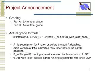
Project Announcement • Grading: • Part A: 3/4 of total grade • Part B: 1/4 of total grade • Actual grade formula: • 3/4*(Max(A1, 0.7*A2)) + 1/4*(Max(B_self, 0.9B_with_staff_code))) • A1 is submission for P1a on or before the part A deadline. • A2 is version of P1a submitted *any time* before the part B deadline. • B_self is part B running against your own implementation of LSP • 0.9*B_with_staff_code is part B running against the reference LSP
15-440 Distributed Systems Lecture 13 – RAID Thanks to Greg Ganger and Remzi Arapaci-Dusseau for slides
Outline • Using multiple disks • Why have multiple disks? • problem and approaches • RAID levels and performance • Estimating availability
Motivation: Why use multiple disks? • Capacity • More disks allows us to store more data • Performance • Access multiple disks in parallel • Each disk can be working on independent read or write • Overlap seek and rotational positioning time for all • Reliability • Recover from disk (or single sector) failures • Will need to store multiple copies of data to recover • So, what is the simplest arrangement?
Just a bunch of disks (JBOD) • Yes, it’s a goofy name • industry really does sell “JBOD enclosures”
Disk Subsystem Load Balancing • I/O requests are almost never evenly distributed • Some data is requested more than other data • Depends on the apps, usage, time, ... • What is the right data-to-disk assignment policy? • Common approach: Fixed data placement • Your data is on disk X, period! • For good reasons too: you bought it or you’re paying more... • Fancy: Dynamic data placement • If some of your files are accessed a lot, the admin(or even system) may separate the “hot” files across multiple disks • In this scenario, entire files systems (or even files) are manually moved by the system admin to specific disks • Alternative: Disk striping • Stripe all of the data across all of the disks
Disk Striping • Interleave data across multiple disks • Large file streaming can enjoy parallel transfers • High throughput requests can enjoy thorough load balancing • If blocks of hot files equally likely on all disks (really?)
Disk striping details • How disk striping works • Break up total space into fixed-size stripe units • Distribute the stripe units among disks in round-robin • Compute location of block #B as follows • disk# = B%N (%=modulo,N = #ofdisks) • LBN# = B / N (computes the LBN on given disk)
Now, What If A Disk Fails? • In a JBOD (independent disk) system • one or more file systems lost • In a striped system • a part of each file system lost • Backups can help, but • backing up takes time and effort • backup doesn’t help recover data lost during that day • Any data loss is a big deal to a bank or stock exchange
Tolerating and masking disk failures • If a disk fails, it’s data is gone • may be recoverable, but may not be • To keep operating in face of failure • must have some kind of data redundancy • Common forms of data redundancy • replication • erasure-correcting codes • error-correcting codes
Redundancy via replicas • Two (or more) copies • mirroring, shadowing, duplexing, etc. • Write both, read either
Mirroring & Striping • Mirror to 2 virtual drives, where each virtual drive is really a set of striped drives • Provides reliability of mirroring • Provides striping for performance (with write update costs)
Implementing Disk Mirroring • Mirroring can be done in either software or hardware • Software solutions are available in most OS’s • Windows2000, Linux, Solaris • Hardware solutions • Could be done in Host Bus Adaptor(s) • Could be done in Disk Array Controller
Lower Cost Data Redundancy • Single failure protecting codes • general single-error-correcting code is overkill • General code finds error and fixes it • Disk failures are self-identifying (a.k.a. erasures) • Don’t have to find the error • Fact: N-error-detecting code is also N-erasure-correcting • Error-detecting codes can’t find an error,just know its there • But if you independently know where error is, allows repair • Parity is single-disk-failure-correcting code • recall that parity is computed via XOR • it’s like the low bit of the sum
Simplest approach: Parity Disk • One extra disk • All writes update parity disk • Potential bottleneck
The parity disk bottleneck • Reads go only to the data disks • But, hopefully load balanced across the disks • All writes go to the parity disk • And, worse, usually result in Read-Modify-Write sequence • So, parity disk can easily be a bottleneck
Solution: Striping the Parity • Removes parity disk bottleneck
Outline • Using multiple disks • Why have multiple disks? • problem and approaches • RAID levels and performance • Estimating availability
RAID Taxonomy • Redundant Array of Inexpensive Independent Disks • Constructed by UC-Berkeley researchers in late 80s (Garth) • RAID 0 – Coarse-grained Striping with no redundancy • RAID 1 – Mirroring of independent disks • RAID 2 – Fine-grained data striping plus Hamming code disks • Uses Hamming codes to detect and correct multiple errors • Originally implemented when drives didn’t always detect errors • Not used in real systems • RAID 3 – Fine-grained data striping plus parity disk • RAID 4 – Coarse-grained data striping plus parity disk • RAID 5 – Coarse-grained data striping plus striped parity • RAID 6 – Coarse-grained data striping plus 2 striped codes
RAID-0: Striping • Stripe blocks across disks in a “chunk” size • How to pick a reasonable chunk size? 0 4 1 5 2 6 3 7 8 12 9 13 10 14 11 15 How to calculate where chunk # lives? Disk: Offset within disk:
RAID-0: Striping • Evaluate for D disks • Capacity: How much space is wasted? • Performance: How much faster than 1 disk? • Reliability: More or less reliable than 1 disk? 0 4 1 5 2 6 3 7 8 12 9 13 10 14 11 15
RAID-1: Mirroring • Motivation: Handle disk failures • Put copy (mirror or replica) of each chunk on another disk 0 2 0 2 1 3 1 3 4 6 4 6 5 7 5 7 Capacity: Reliability: Performance:
RAID-4: Parity • Motivation: Improve capacity • Idea: Allocate parity block to encode info about blocks • Parity checks all other blocks in stripe across other disks • Parity block = XOR over others (gives “even” parity) • Example: 0 1 0 Parity value? • How do you recover from a failed disk? • Example: x 0 0 and parity of 1 • What is the failed value? 0 3 1 4 2 5 P0 P1 6 9 7 10 8 11 P2 P3
RAID-4: Parity • Capacity: • Reliability: • Performance: • Reads • Writes: How to update parity block? • Two different approaches • Small number of disks (or large write): • Large number of disks (or small write): • Parity disk is the bottleneck 0 3 1 4 2 5 P0 P1 6 9 7 10 8 11 P2 P3
RAID-5: Rotated Parity • Capacity: • Reliability: • Performance: • Reads: • Writes: • Still requires 4 I/Os per write, but not always to same parity disk Rotate location of parity across all disks 0 3 1 4 2 P1 P0 5 6 P3 P2 9 7 10 8 11
Advanced Issues • What happens if more than one fault? • Example: One disk fails plus “latent sector error” on another • RAID-5 cannot handle two faults • Solution: RAID-6 (e.g., RDP) Add multiple parity blocks • Why is NVRAM useful? • Example: What if update 2, don’t update P0 before power failure (or crash), and then disk 1 fails? • NVRAM solution: Use to store blocks updated in same stripe • If power failure, can replay all writes in NVRAM • Software RAID solution: Perform parity scrub over entire disk 0 3 1 4 2’ 5 P0 P1 6 9 7 10 8 11 P2 P3
Outline • Using multiple disks • Why have multiple disks? • problem and approaches • RAID levels and performance • Estimating availability
Sidebar: Availability metric • Fraction of time that server is able to handle requests • Computed from MTBF and MTTR (Mean Time To Repair)
How often are failures? • MTBF (Mean Time Between Failures) • MTBFdisk~ 1,200,00 hours (~136 years, <1% per year) • MTBFmutli-disk system = mean time to first disk failure • which is MTBFdisk / (number of disks) • For a striped array of 200 drives • MTBFarray= 136 years / 200 drives = 0.65 years
Reliability without rebuild • 200 data drives with MTBFdrive • MTTDLarray= MTBFdrive / 200 • Add 200 drives and do mirroring • MTBFpair= (MTBFdrive / 2) + MTBFdrive = 1.5 * MTBFdrive • MTTDLarray= MTBFpair / 200 = MTBFdrive / 133 • Add 50 drives, each with parity across 4 data disks • MTBFset= (MTBFdrive / 5) + (MTBFdrive / 4) = 0.45 * MTBFdrive • MTTDLarray= MTBFset / 50 = MTBFdrive / 111
Rebuild: restoring redundancy after failure • After a drive failure • data is still available for access • but, a second failure is BAD • So, should reconstruct the data onto a new drive • on-line spares are common features of high-end disk arrays • reduce time to start rebuild • must balance rebuild rate with foreground performance impact • a performance vs. reliability trade-offs • How data is reconstructed • Mirroring: just read good copy • Parity: read all remaining drives (including parity) and compute
Reliability consequences of adding rebuild • No data loss, if fast enough • That is, if first failure fixed before second one happens • New math is... • MTTDLarray = MTBFfirstdrive * (1 / prob of 2nd failure before repair) • ... which is MTTRdrive / MTBFseconddrive • For mirroring • MTBFpair = (MTBFdrive / 2) * (MTBFdrive / MTTRdrive) • For 5-disk parity-protected arrays • MTBFset = (MTBFdrive / 5) * ((MTBFdrive / 4 )/ MTTRdrive)
Three modes of operation • Normal mode • everything working; maximum efficiency • Degraded mode • some disk unavailable • must use degraded mode operations • Rebuild mode • reconstructing lost disk’s contents onto spare • degraded mode operations plus competition with rebuild
Mechanics of rebuild • Background process • use degraded mode read to reconstruct data • then, write it to replacement disk • Implementation issues • Interference with foreground activity and controlling rate • Rebuild is important for reliability • Foreground activity is important for performance • Using the rebuilt disk • For rebuilt part, reads can use replacement disk • Must balance performance benefit with rebuild interference
Conclusions • RAID turns multiple disks into a larger, faster, more reliable disk • RAID-0: StripingGood when performance and capacity really matter, but reliability doesn’t • RAID-1: MirroringGood when reliability and write performance matter, but capacity (cost) doesn’t • RAID-5: Rotating ParityGood when capacity and cost matter or workload is read-mostly • Good compromise choice