James PM Syvitski & Eric WH Hutton, CSDMS, CU-Boulder

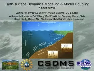
1. Earth-surface Dynamics Modeling & Model Coupling A short course James PM Syvitski & Eric WH Hutton, CSDMS, CU-Boulder With special thanks to Pat Wiberg, Carl Friedrichs, Courtney Harris, Chris Reed, Rocky Geyer, Alan Niedoroda, Rich Signell, Chris Sherwood

2. Module 5: Shelf Sediment Transport ref: Syvitski, J.P.M. et al., 2007. Prediction of margin stratigraphy. In: C.A. Nittrouer, et al. (Eds.) Continental-Margin Sedimentation: From Sediment Transport to Sequence Stratigraphy. IAS Spec. Publ. No. 37: 459-530. Shelf diffusivity (3) Gravity-driven slope equilibrium (4) Event-based models (7) Coastal Ocean Models (4) Summary (1) Earth-surface Dynamic Modeling & Model Coupling, 2009

3. Shelf diffusivity Local transport occurs if the probability of wave resuspension is exceeded at a particle’s water depth. 20000 NDBC Buoy 46022, 1982-1998 1 across shelf along shelf u >50 cm/s bs u >35 cm/s bs 15000 0.8 u >25 cm/s bs u >15 cm/s bs 0.6 10000 Sediment diffusivity (m2/hr) Exceedance Probability 0.4 5000 Eel 0.2 0 40 50 60 70 80 90 100 0 Depth (m) 20 30 40 50 60 70 80 90 100 120 150 Water Depth (m) Earth-surface Dynamic Modeling & Model Coupling, 2009

4. Shelf diffusivity Resuspension and Advection by Bottom Boundary Energy • k(t,z) varies over time t (pdf of storms), and water depth z. Following Airy wave theory, k falls off exponentially with water depth. • ki is an index between 0 and 1 that reflects the ability of grain size i to be resuspended and advected. • k(t,z) ≥ ki for sediment transport Earth-surface Dynamic Modeling & Model Coupling, 2009

5. Plumes Only Plumes & Wave Diffusion Earth-surface Dynamic Modeling & Model Coupling, 2009

6. Gravity-driven slope equilibrium density stratification Shear instabilities occur for Ri < Ricr “ “ suppressed for Ri > Ricr Gradient Richardson Number (Ri) = velocity shear (b) (a) Height above bed Height above bed Ri > Ricr Ri = Ricr Ri = Ricr Ri < Ricr Sediment concentration Sediment concentration • If excess sediment enters BBL & Ri increases beyond Ricr, then turbulence is dampened, sediment is deposited, stratification is reduced and Ri returns to Ricr • If excess sediment settles out of boundary layer, or bottom stress increases & Ri decreases beyond Ricr then turbulence intensifies. Sediment re-enters base of boundary layer. Stratification is increased in boundary layer and Ri returns to Ricr. Earth-surface Dynamic Modeling & Model Coupling, 2009

7. Gravity-driven slope equilibrium Buoyancy Shear z z = h c' z = 0 y q x a B = cd < |u| u > Down-slope pressure gradient = Bottom friction = (Uw2 + vc2+ugrav2)1/2 total velocity Richardson Number = = Critical value (Wright et al., Mar.Geol. 2001) (i) Momentum balance: = cd Umax ugrav x-shelf bed slope x-shelf gravity flow velocity wave-averaged, x-shelf component of quadratic velocity depth-integrated buoyancy anomaly bottom drag coefficient (ii) Maximum turbulent sediment load: (c.f. Trowbridge & Kineke, JGR 1994) Earth-surface Dynamic Modeling & Model Coupling, 2009

8. COMPARISON OF MODEL PREDICTIONS TO OBSERVED DEPOSITION Application to 1996-97 Eel River Flood at 60-meter Site Deposition Rate Porosity (rsed/rwater -1) Bed slope Richardson # Drag coeff. P = 0.9 s = 1.6 a = 0.004 Ricr = 0.25 cd = 0.003 (Observations from Traykovski et al., CSR 2000) Wave orbital velocity Suspended sediment Predicted bed elevation Observed bed elevation Earth-surface Dynamic Modeling & Model Coupling, 2009

9. Top: Plumes & Wave Diffusion; Bottom: Plumes, Waves & Fluid Muds Earth-surface Dynamic Modeling & Model Coupling, 2009

10. qs Surface active layer Mixed layer  Exchange layer (after Parker) Event-based transport model Calculate suspended sediment flux (by grain size) using a 1-D shelf sediment transport model at a cross-shelf grid of nodes of specified depth and sediment characteristics. For each event (set of wave & current conditions), the net flux is calculated at each node. The divergence of the flux gives the change in bed elevation. Earth-surface Dynamic Modeling & Model Coupling, 2009

11. 5 Bed elevation (cm) 0 -5 4 6 8 10 12 14 16 1 m <45 m m 45-63 m m 63-125 m Silt fraction 0.5 m 125-500 m 0 4 6 8 10 12 14 16 1 0.5 Sand fraction 0 4 6 8 10 12 14 16 Cross-shelf distance (km) Example of 5 repetitions of a transport event on Eel Margin. Earth-surface Dynamic Modeling & Model Coupling, 2009

12. SLICE Description SLICE Description wind tides waves grid Neidoroda & Reed Earth-surface Dynamic Modeling & Model Coupling, 2009

13. Neidoroda & Reed SLICE Description Earth-surface Dynamic Modeling & Model Coupling, 2009

14. Neidoroda & Reed SLICE Density Flows Mudflow Profile Mudflow Deposit Earth-surface Dynamic Modeling & Model Coupling, 2009

15. Neidoroda & Reed Earth-surface Dynamic Modeling & Model Coupling, 2009

16. Neidoroda & Reed Earth-surface Dynamic Modeling & Model Coupling, 2009

17. Nested Modeling Average Sediment and Currents. Sept, 2002 – May, 2003 C.Harris, VIMS C.Harris, VIMS Regional Hydrological Model (HydroTrend) (atm-landsurface model) to Regional Ocean Model (ROMS) for Sediment Supply, Buoyancy, Sediment Plumes Global Ocean Model (NOGAPS) (coupled ocean-atm model) to Regional Ocean Model (ROMS) (coupled ocean-atm model) for Regional Circulation and Current Shear Global Met. Model (NOGAPS) (coupled ocean-atm model) to Regional Met. Model (COAMPS) (coupled ocean-atm model) to Wave Model (SWAN) for Sediment Resuspension (ROMS) Earth-surface Dynamic Modeling & Model Coupling, 2009

18. Circulation and Sediment-Transport Modeling • ROMS: Regional Ocean Modeling System — RANS for heat & momentum fluxes • 3-8 km grid, 21 vertical “S” levels • Initialized with ship data • Zero-gradient b.c. near Otronto, seven tidal components • LAMI forcing every 3 hours, SWAN waves, Po River discharge • k-w turbulence model, Styles & Glenn wave-current boundary layer • Resuspension & transport of single grain size, ws = 0.1 mm/s, tc =0.08Pa Salinity; Depth-meancurrents Winds; Wave height Bottom currents; Sus. Seds. Earth-surface Dynamic Modeling & Model Coupling, 2009

19. C. Sherwood, USGS Earth-surface Dynamic Modeling & Model Coupling, 2009

20. 2 km Sediment Model Inputs: sediment sources, sizes, critical shear stress, settling velocity. Calculates: flux, concentration, erosion / deposition. Currents, Bed Shear Sea Floor Grid VIMS-NCOM 3D Transport Model NCOM Vertical Grid Earth-surface Dynamic Modeling & Model Coupling, 2009

21. Conclusions: Shelf diffusivity Advantages: uses daily pdf of regional ocean energy, simple and robust; compatible with landscape evolution models Disadvantages: depends wave energy pdf -- how variable is diffusion in response to decadal and longer term variability? Gravity-driven slope equilibrium Advantages: uses daily pdf of local total velocity, simple and robust; can be tested against field data Disadvantages: Needs pdf for wave energy and sediment discharge from rivers, to calculate Richardson number Event-based Approach Advantages: uses wave, current, and sediment information available for a site, preserving all correlations, can be tested against field data Disadvantages: time scales short, data needs intensive for long-term simulations, inshore boundary condition difficult to specify Coastal Ocean Model Advantages: Can get it right if all terms are included & appropriate resolution is used. Disadvantage: Computationally intensive: data needs intensive Earth-surface Dynamic Modeling & Model Coupling, 2009