Download
1 / 27
280 likes | 407 Vues
Primal-Dual Algorithms for Connected Facility Location. Chaitanya Swamy Amit Kumar Cornell University. Connected Facility Location (ConFL). Graph G=(V,E) , costs {c e } on edges and a parameter M ≥ 1. F : set of facilities . D : set of clients ( demands ).

E N D
Primal-Dual Algorithms for Connected Facility Location Chaitanya Swamy Amit Kumar Cornell University
Connected Facility Location (ConFL) Graph G=(V,E), costs {ce} on edges and a parameter M ≥ 1. F : set of facilities. D : set of clients(demands). Facility i has facility costfi. cij : distance between i and j in V. facility client node ALADDIN Workshop, 10/2002
Pick a set A of facilities to open. • Assign each demand j to an open facility i(j). • Connect all open facilities by a Steiner treeT. open facility facility client Steiner tree We want to : Cost=iÎA fi+jÎD ci(j)j+M eÎT ce =facility opening cost+ client assignment cost +cost of connecting facilities. ALADDIN Workshop, 10/2002
Previous Work • Ravi & Selman : Look at related problem - connect facilities by a tour. Round optimal solution of an exponential size LP. • Karger & Minkoff : Combinatorial algorithm with ‘large’ constant approx. ratio. • Gupta, Kleinberg, Kumar, Rastogi & Yener : Also use LP rounding. Get a 9.001-approx. if F =V, fi = 0 for all i, a 10.66-approx. in the general case. • Guha, Meyerson & Munagala; Talwar : Gave a constant approx. for the single-sink buy-at-bulk problem. ALADDIN Workshop, 10/2002
Our Results • Give primal-dual algorithms with approx. ratios of 5 (F =V, fi = 0) and 9 (general case). • Use this to solve the Connected k-Median problem, and an edge capacitated version of ConFL. ALADDIN Workshop, 10/2002
Rent-or-buy problem Special case with F =V and fi = 0,"i. Suppose we know a facility f that is open in an optimal solution. What does the solution look like ? Open facility f Steiner tree. : cost of e = Mce. Shortest paths : cost of e = ce(demand through e). ALADDIN Workshop, 10/2002
Equivalently, Want to route traffic from clients to f by installing capacity on edges. 2 choices : I : Rent Capacity cost µrented capacity (Shortest Paths) II : Buy Capacity fixed cost, ∞ capacity (Steiner Tree) cost cost M capacity capacity ConFLºsingle-sink buy-at-bulk problem with 2 cable types and sinkf. ALADDIN Workshop, 10/2002
C*, S* : assignment, Steiner cost of OPT. OPT S* Total cost of adding edges ≤C*+C. C* Opt. Steiner tree on ≤S*+C*+C. ÞS ≤ 2(S*+C*+C) Þget an O(1)-approx. Design Guideline Cluster enough demandat a facility before opening it. Suppose we run a g-approx. algorithm for FL, and each open facility serves ≥ M clients. C ≥ M ALADDIN Workshop, 10/2002
f S j An Integer Program xij = 1if demandjis assigned toi. ze = 1if edgeeis included in the Steiner tree. • Min.j,i cijxij + Me ceze(primal) • s.t. • i xij≥ 1 j • iÎS xij ≤ eÎ(S)ze • S ÍV : fÏS, j • xij, ze Î {0, 1} (1) Relax (1) to xij, ze≥ 0 to get an LP. ALADDIN Workshop, 10/2002
f S:eÎd(S),fÏS yS ≤ Mce cij Max. j vj j Any feasible dual solution is a lower bound on OPT–Weak Duality. What is the dual? vjº amount j is willing to ‘pay’ to route its demand to f. Let yS = j yS,j. {yS }º moat packing around facilities. vj ≤ cij + S:iÎS,fÏS yS,j ALADDIN Workshop, 10/2002
The Algorithm • Decide which facilities to open, cluster demands around open facilities. Construct a primal soln. and dual soln. (v,y) simultaneously. • Build a Steiner tree on open facilities. • The following will hold after 1) : • (v,y) is a feasible dual solution. • j is assigned to i(j) s.t. ci(j)j ≤ 3vj. • Each open facility i has ≥ M clients, {j}, assigned to it s.t. cij ≤ vj. ALADDIN Workshop, 10/2002
can amortize thecost against demands in Di. Di ≥ M i So, S ≤ 2(S*+ C*+ jÎD1 vj). Analysis Suppose the 3 properties hold. Let A be the set of facilities opened, Di= {j assigned to i : cij ≤ vj } for iÎA. Then, |Di| ≥ M. Let D1= UiÎA Di. C ≤ jÎD1 vj + jÏD1 3vj. ALADDIN Workshop, 10/2002
C*, S* : assignment, Steiner cost of OPT. OPT S* Total cost of adding edges ≤C*+C. C* Opt. Steiner tree on ≤S*+C*+C. ÞS ≤ 2(S*+C*+C) Þget an O(1)-approx. Design Guideline Cluster enough demandat a facility before opening it. Suppose we run a g-approx. algorithm for FL, and each open facility serves ≥ M clients. C ≥ M ALADDIN Workshop, 10/2002
can amortize thecost against demands in Di. Di ≥ M i So, S ≤ 2(S*+ C*+ jÎD1 vj). Total cost ≤2(S*+ C*) + 3 jÎD vj ≤ 5 OPT. Analysis Suppose the 3 properties hold. Let A be the set of facilities opened, Di= {j assigned to i : cij ≤ vj } for iÎA. Then, |Di| ≥ M. Let D1= UiÎA Di. C ≤ jÎD1 vj + jÏD1 3vj. ALADDIN Workshop, 10/2002
Phase 1 Simplifying assumption – can open a facility anywhere along an edge. locations Notion of time, t. Start at t=0. Initially vj = 0, j. f is tentatively open, all other locations are closed. Say j is tight with i (has reached i) if vj ≥ cij. Sj is set of vertices j is tight with. ALADDIN Workshop, 10/2002
Raise all vj at rate 1. Also raise ySj,j at same rate. • Keep raising vjs until : • There is a closed location i with which M demands become tight : tentatively openi. Freeze all these M demands. • j reaches a tentatively open location : freezej. Now only raise vj of unfrozen demands. Continue this process until all demands are frozen. ALADDIN Workshop, 10/2002
M=2, time t=1 tentatively open location not open location unfrozen demand Execution of the algorithm M=2, time t=0 f ALADDIN Workshop, 10/2002
frozen demand Execution of the algorithm M=2, time t=2 f tentatively open location not open location unfrozen demand ALADDIN Workshop, 10/2002
tentatively open location not open location unfrozen demand frozen demand Execution of the algorithm M=2, time t=3 f vj=t=3 j ALADDIN Workshop, 10/2002
Say i, l are dependent if Di Ç Dl¹ f. Pick an indepdt. set of locations, A ÍA’ and open these. Initially A =f. Consider locations in order of ti. If A U {i} is independent add i to A. Here order is 0,1,2,3,4 so A={0,1,3}. Opening locations • Let i be tentatively open. • Di= {j : j is tight with i }. • ti= time when i was tent’vely opened. • Note, |Di|≥M. But the Dis may not be disjoint. 2 f 0 1 3 4 ALADDIN Workshop, 10/2002
j is tight with some open i : assign j to i. At most 1 open i may be tight with j. 1) i j 2) tentatively open location, not open i j l k open location i is tentatively open and caused j to get frozen Þ j is tight with i. i and l are dependent, tl ≤ ti and l is open : assign j to l. Assigning clients Consider client j. ALADDIN Workshop, 10/2002
i(j) = location that j is assigned to. • ci(j)j ≤ vj. • ci(j)j ≤ vj+ 2vk. • vj ≥ ti since j freezes at or after time ti. • Also vk ≤ ti. • So vk ≤ vj and ci(j)j ≤ 3vj. For every open i, all clients in Di are assigned to i. |Di| ≥ M, so at leastMdemands{j}are assigned toiwithcij ≤ vj. ALADDIN Workshop, 10/2002
vj ≤ cij + S:iÎS,fÏS yS,j Once j reaches i, set Sjincludes i and ySj,j is increasing at same rate as vj. vj j cij i Sj j S:eÎd(S),fÏS yS,j ≤ Mce M=3 j(S yS,j) = pÎe(#of across p) ≤ pÎe M = Mce. e ≤ M at any location Putting it together Need to show that (v,y) is feasible. ALADDIN Workshop, 10/2002
Done? Almost… Could have opened non-vertex locations. Fix : Move all such locations to vertices. Cost only decreases ! e.g., ≥ M Theorem : The above algorithm is a 5-approx. for rent-or-buy. ALADDIN Workshop, 10/2002
The General Case • FÍ V : Cannot open a facility everywhere. • Facilities have costs : Want to open cheap facilities. • Modified Phase 1 • Dual variables, vj, also pay for opening facilities. • Cluster ≥M demands around terminal locations, open facilities ‘near’ terminal locations. Theorem : There is a 9-approx. algorithm for the general case. ALADDIN Workshop, 10/2002
open facility 2(S*+ C*+ jÎD1 vj). Total cost ≤2(S*+ C*) + 7 jÎD vj ≤ 9 OPT. Let A be the set of terminal locations, Di= {j : cij ≤ vj } for iÎA. We ensure |Di| ≥ M. Let D1= UiÎA Di. Can show, F + C ≤ jÎD1 3vj + jÏD1 7vj. ≤2 minjÎDi vj Di ≥ M i S ≤ jÎD1 2vj + ALADDIN Workshop, 10/2002
Open Questions • Better approximation : only know an integrality gap of 2 from Steiner tree. • Multicommodity buy-at-bulk.Multiple source-sink pairs, route flow from source to sink. Have different cable types. Kumar et al. give a const. approx. for multicommodity rent-or-buy. • Unrelated metrics : Min.i fiyi + j,i cijxij + e deze. Can reduce from group Steiner tree – get a O(log2 n) LB. Matching UB? ALADDIN Workshop, 10/2002