Data Warehouses and OLAP

1. Data Warehouses and OLAP *Slides by Nikos Mamoulis

2. other sources Extract Transform Load Refresh Operational DBs Multi-Tiered Architecture Monitor & Integrator OLAP Server Metadata Analysis Query Reports Data mining Serve Data Warehouse Data Marts Data Sources Data Storage OLAP Engine Front-End Tools

3. OLAP Server Architectures • Relational OLAP (ROLAP) • Use relational or extended-relational DBMS to store and manage warehouse data and OLAP middle ware to support missing pieces • Include optimization of DBMS backend, implementation of aggregation navigation logic, and additional tools and services • greater scalability • Multidimensional OLAP (MOLAP) • Array-based multidimensional storage engine (sparse matrix techniques) • fast indexing to pre-computed summarized data • Hybrid OLAP (HOLAP) • User flexibility, e.g., low level: relational, high-level: array • Specialized SQL servers • specialized support for SQL queries over star/snowflake schemas

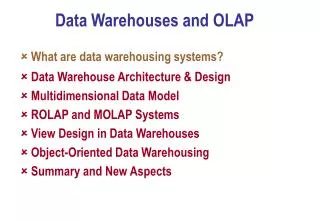
4. Data Warehousing and OLAP Technology for Data Mining • What is a data warehouse? • A multi-dimensional data model • Data warehouse architecture • Data warehouse implementation • Further development of data cube technology • From data warehousing to data mining

5. Efficient Data Cube Computation • Data cube can be viewed as a lattice of cuboids • The bottom-most cuboid is the base cuboid • The top-most cuboid (apex) contains only one cell • How many cuboids in an n-dimensional cube with L levels? • Materialization of data cube • Materialize every (cuboid) (full materialization), none (no materialization), or some (partial materialization) • Selection of which cuboids to materialize • Based on size, sharing, access frequency, etc.

6. Cube Operations • Cube definition and computation in DMQL define cube sales[item, city, year]: sum(sales_in_dollars) compute cube sales • Transform it into a SQL-like language (with a new operator cube by, introduced by Gray et al.’96) SELECT item, city, year, SUM (amount) FROM SALES CUBE BY item, city, year • Need compute the following Group-Bys (date, product, customer), (date,product),(date, customer), (product, customer), (date), (product), (customer) () () (city) (item) (year) (city, item) (city, year) (item, year) (city, item, year)

7. Cube Computation: ROLAP-Based Method • Efficient cube computation methods • ROLAP-based cubing algorithms (Agarwal et al’96) • Array-based cubing algorithm (Zhao et al’97) • Bottom-up computation method (Bayer & Ramarkrishnan’99) • ROLAP-based cubing algorithms • Sorting, hashing, and grouping operations are applied to the dimension attributes in order to reorder and cluster related tuples • Grouping is performed on some sub-aggregates as a “partial grouping step” • Aggregates may be computed from previously computed aggregates, rather than from the base fact table

8. C c3 61 62 63 64 c2 45 46 47 48 c1 29 30 31 32 c 0 B 60 13 14 15 16 b3 44 28 56 9 b2 B 40 24 52 5 b1 36 20 1 2 3 4 b0 a0 a1 a2 a3 A Multi-way Array Aggregation for Cube Computation • Partition arrays into chunks (a small subcube which fits in memory). • Compressed sparse array addressing: (chunk_id, offset) • Compute aggregates in “multiway” by visiting cube cells in the order which minimizes the # of times to visit each cell, and reduces memory access and storage cost. What is the best traversing order to do multi-way aggregation?

9. C c3 61 62 63 64 c2 45 46 47 48 c1 29 30 31 32 c 0 B 60 13 14 15 16 b3 44 28 56 9 b2 40 24 52 5 b1 36 20 1 2 3 4 b0 a0 a1 a2 a3 A Multi-way Array Aggregation for Cube Computation B

10. Multi-way Array Aggregation for Cube Computation C c3 61 62 63 64 c2 45 46 47 48 c1 29 30 31 32 c 0 B 60 13 14 15 16 b3 44 28 B 56 9 b2 40 24 52 5 b1 36 20 1 2 3 4 b0 a0 a1 a2 a3 A

11. Multi-Way Array Aggregation for Cube Computation (Cont.) • Method: the planes should be sorted and computed according to their size in ascending order. • See the details of Example 4.4 • Idea: keep the smallest plane in the main memory, fetch and compute only one chunk at a time for the largest plane • Limitation of the method: works well only for a small number of dimensions • If there are a large number of dimensions, “bottom-up computation” and iceberg cube computation methods can be explored

12. Indexing OLAP Data: Bitmap Index • Index on a particular column • Each value in the column has a bit vector: bit-op is fast • The length of the bit vector: # of records in the base table • The i-th bit is set if the i-th row of the base table has the value for the indexed column • not suitable for high cardinality domains Base table Index on Region Index on Type

13. Indexing OLAP Data: Join Indices • Join index: JI(R-id, S-id) where R (R-id, …)  S (S-id, …) • Traditional indices map the values to a list of record ids • It materializes relational join in JI file and speeds up relational join — a rather costly operation • In data warehouses, join index relates the values of the dimensions of a start schema to rows in the fact table. • E.g. fact table: Sales and two dimensions city and product • A join index on city maintains for each distinct city a list of R-IDs of the tuples recording the Sales in the city • Join indices can span multiple dimensions

14. Efficient Processing OLAP Queries • Determine which operations should be performed on the available cuboids: • transform drill, roll, etc. into corresponding SQL and/or OLAP operations, e.g, dice = selection + projection • Determine to which materialized cuboid(s) the relevant operations should be applied. • Exploring indexing structures and compressed vs. dense array structures in MOLAP

15. Metadata Repository • Meta data is the data defining warehouse objects. It has the following kinds • Description of the structure of the warehouse • schema, view, dimensions, hierarchies, derived data defn, data mart locations and contents • Operational meta-data • data lineage (history of migrated data and transformation path), currency of data (active, archived, or purged), monitoring information (warehouse usage statistics, error reports, audit trails) • The algorithms used for summarization • The mapping from operational environment to the data warehouse • Data related to system performance • warehouse schema, view and derived data definitions • Business data • business terms and definitions, ownership of data, charging policies

16. Data Warehouse Back-End Tools and Utilities • Data extraction: • get data from multiple, heterogeneous, and external sources • Data cleaning: • detect errors in the data and rectify them when possible • Data transformation: • convert data from legacy or host format to warehouse format • Load: • sort, summarize, consolidate, compute views, check integrity, and build indicies and partitions • Refresh • propagate the updates from the data sources to the warehouse

17. Data Warehousing and OLAP Technology for Data Mining • What is a data warehouse? • A multi-dimensional data model • Data warehouse architecture • Data warehouse implementation • Further development of data cube technology • From data warehousing to data mining

18. Discovery-Driven Exploration of Data Cubes • Hypothesis-driven: exploration by user, huge search space • Discovery-driven (Sarawagi et al.’98) • pre-compute measures indicating exceptions, guide user in the data analysis, at all levels of aggregation • Exception: significantly different from the value anticipated, based on a statistical model • Visual cues such as background color are used to reflect the degree of exception of each cell • Computation of exception indicator (modeling fitting and computing SelfExp, InExp, and PathExp values) can be overlapped with cube construction

19. Examples: Discovery-Driven Data Cubes

20. Data Warehousing and OLAP Technology for Data Mining • What is a data warehouse? • A multi-dimensional data model • Data warehouse architecture • Data warehouse implementation • Further development of data cube technology • From data warehousing to data mining

21. Data Warehouse Usage • Three kinds of data warehouse applications • Information processing • supports querying, basic statistical analysis, and reporting using crosstabs, tables, charts and graphs • Analytical processing • multidimensional analysis of data warehouse data • supports basic OLAP operations, slice-dice, drilling, pivoting • Data mining • knowledge discovery from hidden patterns • supports associations, constructing analytical models, performing classification and prediction, and presenting the mining results using visualization tools. • Differences among the three tasks

22. From On-Line Analytical Processing to On Line Analytical Mining (OLAM) • Why online analytical mining? • High quality of data in data warehouses • DW contains integrated, consistent, cleaned data • Available information processing structure surrounding data warehouses • ODBC, OLEDB, Web accessing, service facilities, reporting and OLAP tools • OLAP-based exploratory data analysis • mining with drilling, dicing, pivoting, etc. • On-line selection of data mining functions • integration and swapping of multiple mining functions, algorithms, and tasks. • Architecture of OLAM

23. An OLAM Architecture Mining query Mining result Layer4 User Interface User GUI API OLAM Engine OLAP Engine Layer3 OLAP/OLAM Data Cube API Layer2 MDDB MDDB Meta Data Database API Filtering&Integration Filtering Layer1 Data Repository Data cleaning Data Warehouse Databases Data integration

24. Summary • Data warehouse • A subject-oriented, integrated, time-variant, and nonvolatile collection of data in support of management’s decision-making process • A multi-dimensional model of a data warehouse • Star schema, snowflake schema, fact constellations • A data cube consists of dimensions & measures • OLAP operations: drilling, rolling, slicing, dicing and pivoting • OLAP servers: ROLAP, MOLAP, HOLAP • Efficient computation of data cubes • Partial vs. full vs. no materialization • Multiway array aggregation • Bitmap index and join index implementations • Further development of data cube technology • Discovery-drive and multi-feature cubes • From OLAP to OLAM (on-line analytical mining)

25. References (I) • S. Agarwal, R. Agrawal, P. M. Deshpande, A. Gupta, J. F. Naughton, R. Ramakrishnan, and S. Sarawagi. On the computation of multidimensional aggregates. In Proc. 1996 Int. Conf. Very Large Data Bases, 506-521, Bombay, India, Sept. 1996. • D. Agrawal, A. E. Abbadi, A. Singh, and T. Yurek. Efficient view maintenance in data warehouses. In Proc. 1997 ACM-SIGMOD Int. Conf. Management of Data, 417-427, Tucson, Arizona, May 1997. • R. Agrawal, J. Gehrke, D. Gunopulos, and P. Raghavan. Automatic subspace clustering of high dimensional data for data mining applications. In Proc. 1998 ACM-SIGMOD Int. Conf. Management of Data, 94-105, Seattle, Washington, June 1998. • R. Agrawal, A. Gupta, and S. Sarawagi. Modeling multidimensional databases. In Proc. 1997 Int. Conf. Data Engineering, 232-243, Birmingham, England, April 1997. • K. Beyer and R. Ramakrishnan. Bottom-Up Computation of Sparse and Iceberg CUBEs. In Proc. 1999 ACM-SIGMOD Int. Conf. Management of Data (SIGMOD'99), 359-370, Philadelphia, PA, June 1999. • S. Chaudhuri and U. Dayal. An overview of data warehousing and OLAP technology. ACM SIGMOD Record, 26:65-74, 1997. • OLAP council. MDAPI specification version 2.0. In http://www.olapcouncil.org/research/apily.htm, 1998. • J. Gray, S. Chaudhuri, A. Bosworth, A. Layman, D. Reichart, M. Venkatrao, F. Pellow, and H. Pirahesh. Data cube: A relational aggregation operator generalizing group-by, cross-tab and sub-totals. Data Mining and Knowledge Discovery, 1:29-54, 1997.

26. References (II) • V. Harinarayan, A. Rajaraman, and J. D. Ullman. Implementing data cubes efficiently. In Proc. 1996 ACM-SIGMOD Int. Conf. Management of Data, pages 205-216, Montreal, Canada, June 1996. • Microsoft. OLEDB for OLAP programmer's reference version 1.0. In http://www.microsoft.com/data/oledb/olap, 1998. • K. Ross and D. Srivastava. Fast computation of sparse datacubes. In Proc. 1997 Int. Conf. Very Large Data Bases, 116-125, Athens, Greece, Aug. 1997. • K. A. Ross, D. Srivastava, and D. Chatziantoniou. Complex aggregation at multiple granularities. In Proc. Int. Conf. of Extending Database Technology (EDBT'98), 263-277, Valencia, Spain, March 1998. • S. Sarawagi, R. Agrawal, and N. Megiddo. Discovery-driven exploration of OLAP data cubes. In Proc. Int. Conf. of Extending Database Technology (EDBT'98), pages 168-182, Valencia, Spain, March 1998. • E. Thomsen. OLAP Solutions: Building Multidimensional Information Systems. John Wiley & Sons, 1997. • Y. Zhao, P. M. Deshpande, and J. F. Naughton. An array-based algorithm for simultaneous multidimensional aggregates. In Proc. 1997 ACM-SIGMOD Int. Conf. Management of Data, 159-170, Tucson, Arizona, May 1997.

27. Selection of tables, attributes, domains in the DW design process • If you are asked to design a data warehouse for a set of operational databases how would you do it? • Use specifications of requirements to design the data warehouse schema and select: • The central theme(s) of the analysis (e.g., sales) • The measures on the central themes (e.g., sum(dollars)) • The dimensions used by analytical processing • The attributes and hierarchies of the dimensions • Clean, transform, and integrate information

28. Example • A large company which sells engine parts • Database 1 (Los Angeles) • employee(id, name, dept, lot, salary, age) • department(id, name, type, manager_id) • part(id, name, type, brand, manufacturer, color) • customer(id, name, type, age, city, state, zip, tel) • sales(id, part_id, customer_id, quantity, price) • Database 2 (New York) • employee(id, ename, dept_id, salary, age) • department(id, name, type, manager) • part(id, title, type, brand, manufacturer, color) • customer(id, name, type, zip, tel) • location(zip, city_id) • city(city_id, state, country) • sales(id, part_id, customer_id, quantity, price)

29. Example: requirements and selection • Requirements of the data warehouse • we want to analyze the total sales in dollars and the average price of sold units with respect to time, part, customer. • Selection of the basic features of the warehouse • central theme(s): sales • measure(s): sum(sales_in_dollars), avg(price_sold_units) • dimensions: time, part, customer

30. Example: selection of hierarchies • To determine the dimension hierarchies we have to select which dimensional attributes are required to include for analysis • We go back to the requirements and ask the analyst: • time: day, week, month, quarter, year • part: name, type, color, brand, manufacturer • customer: name, type, city, state, country

31. Exercise • Find the hierarchies for time, part, customer • time: day, week, month, quarter, year • part: name, type, color, brand, manufacturer • customer: name, type, city, state, country

32. Example: selection of hierarchies • Definition of the hierarchies: year manufacturer country state quarter type color brand type city month week name name day customer part time

33. Example: is the information that we need to analyze available? • We have to check if the required information for analysis exists in the databases to be integrated • All requested attributes exist, except from the time. This can be determined by accessing the transaction logs of the databases.

34. Example: Design the DW schema • We use the star schema in this example Time Fact table Customer Part We need just quantity and (unit) price to derive sum(sales_in_dollars) = quantity*price avg(price_sold_units) = Σ(quantity*price)/ Σ(quantity)

35. Integration tasks • convert: • attribute names • attribute types • A large company which sells engine parts • Database 1 (Los Angeles) • employee(id, name, dept, lot, salary, age) • department(id, name, type, manager_id) • part(id, name, type, brand, manufacturer, color) • customer(id, name, type, age, city, state, zip, tel) • sales(id, part_id, customer_id, quantity, price) • Database 2 (New York) • employee(id, ename, dept_id, salary, age) • department(id, name, type, manager) • part(id, title, type, brand, manufacturer, color) • customer(id, name, type, zip, tel) • location(zip, city_id) • city(city_id, state, country) • sales(id, part_id, customer_id, quantity, price) join tables derive data not stored explicitly in the databases fill in missing values • ignore irrelevant data: • tables • attributes

36. Example: how to populate the DW?Load, Clean, Integrate • Convert attribute names and types • E.g., part.name = part.title • Convert values to be consistent • Join tables if necessary • Join customer,location,city from “New York” DB • Derive time if not present • Check transaction log for sales table to get the time and convert it to the required format • Complete missing values • The “Los Angeles” database does not record customer country information because all its customers are from US. In the integrated data from LA country value is set to “USA” • Ignore irrelevant tables and attributes • Tables employee, department are ignored • Attributes zip, tel, id are ignored.

37. How many cuboids ? • How do we compute the total number of cuboids of a data cube? • Compute the product of the number of levels for each dimension • Number of cuboids = (levels for time)* (levels for part)* (levels for customer) = 5*4*5 = 100

38. What is the data cube? • The data cube is NOT a cube • Multiple dimensions, variable range and interpretations of the cells, does not look always like a “cube” • The data cube is the set of all non-redundand, multidimensional views from which we can analyze the measures on the central theme(s) • Remember: the terms multidimensional view and cuboidhave the same meaning • A multidimensional view is non-redundant, if there are no hierarchical relationships between its dimensional attributes

39. month part_brand 23 12 23 11 50 67 23 12 0 0 0 0 manufacturer 10 20 43 33 13 22 0 0 43 33 13 0 58 18 72 25 30 25 0 0 0 0 0 25 part_type 23 12 0 40 90 12 23 45 43 33 13 1 2 0 56 23 6 25 Redundancy in views • A non-redundant combination of attributes: • (month, part_type) • A redundant (not useful) combination of attributes: • (part_brand, part_manufacturer)

40. Exercise • Find the non-redundant combinations of the attributes of part. manufacturer type color brand name part

41. Visualization of non-redundant attribute combinations for part ALL manufacturer type color brand (type,color) (type, manufacturer) (color, manufacturer) (color,brand) (type,brand) (type,color,manufacturer) (type,color,brand) name part

42. How many (non-redundant) cuboids ? • How do we compute the total number of cuboids of a data cube? • Compute the product of the number of combinations for each dimension • Number of cuboids = (combinations for time)* (combinations for part)* (combinations for customer) = 6*13*9 = 702 • Note: sometimes we use the term cuboid to also denote multidimensional views with selections: • total sales for each (part.type,customer.city) for year = “2001” • We do not count such cuboids in the computation above

43. Cube: A Lattice of Cuboids E.g., (location) is dependent on (time,item,location) all time item location supplier time,item time,location item,location location,supplier time,supplier item,supplier time,location,supplier time,item,location item,location,supplier time,item,supplier time, item, location, supplier

44. How to answer queries from a set of materialized cuboids? • In real-life examples it is not possible to materialize the whole data cube • Typically, a small subset of cuboids is materialized • To answer a query we have to select the cuboid that results in the minimum cost for the query • A query typically consists of • a set of group-by attributes • a set of selection clauses • E.g., compute the total sales per part.type, cust.city for year=2002. • The factors for selecting the best cuboid for a particular query are: • the size of the cuboid • any indexes on the attributes of the “select” clause of the query

45. Cube: A Lattice of Cuboids How would you compute the following queries? Q1: <time,item> Q2: <supplier> Q3: <location> Q4: <time,supplier> Q5: <item> = materialized cuboid all time item location supplier time,item time,location item,location location,supplier time,supplier item,supplier time,location,supplier time,item,location item,location,supplier time,item,supplier time, item, location, supplier

46. Which cuboids should we materialize? • In real-life examples it is not possible to materialize the whole data cube • We have to select the most beneficial cuboids to materialize • This depends mainly on the size of the cuboids and their usage by queries • Thus to select we need information about (i) the size of cuboids, (ii) the queries and their frequency • The base cuboid almost always corresponds to the fact table, which is already materialized. For example, if the products have unique name, and customers unique name, we can use: • time_id to derive the day • part_id to derive part.name • cust_id to derive customer.name

47. Which cuboids should we materialize? • Example • candidate cuboids: • (day,pname,cname) – 100GB (already materialized) • (day,pname) – 60GB • (day,cname) – 20GB • (pname,cname) – 1GB • (day) – 10GB • (pname) – 200MB • (cname) – 30MB • (ALL) – 8 bytes • queries (with equal probability) • Q1: total sales per (pname,cname) • Q2: total sales per (pname) • Q3: total sales per (cname) • Exercise: Which views • should we materialize if • the available space is: • 10GB • 1GB • 100MB

48. Which cuboids should we materialize? • Case 1: Available space = 10GB • We can materialize all three views (pname,cname) , (pname), and (cname) • The cost of Q1 is reading 1GB • The cost of Q2 is reading 200MB • The cost of Q3 is reading 30MB • Average query cost = (1230MB)/3=410 MB/query

49. Which cuboids should we materialize? • Case 2: Available space = 1GB • We have two choices: • materialize (pname,cname) using 1GB • Q1 costs 1GB, Q2 costs 1GB, Q3 costs 1GB • Average query cost = 1GB • materialize (pname) and (cname) using 230MB • Q1 costs 100GB, Q2 costs 200MB, Q3 costs 30MB • Average query cost = (100,230MB)/3 = 34GB • First choice is better than the second!

50. Which cuboids should we materialize? • Case 3: Available space = 100MB • We can only materialize (cname) • Q1 costs 100GB • Q2 costs 100GB • Q3 costs 30MB • Average query cost = (200,030MB)/3 = 67GB