Download
1 / 52
580 likes | 778 Vues
Data Warehouses and OLAP. Based on slides by J Han and C Faloutsos. Data Mining Overview. Data Mining Data warehouses and OLAP (On Line Analytical Processing.) Association Rules Mining Clustering: Hierarchical and Partitional approaches

E N D
Data Warehouses and OLAP Based on slides by J Han and C Faloutsos Data Mining: Concepts and Techniques
Data Mining Overview • Data Mining • Data warehouses and OLAP (On Line Analytical Processing.) • Association Rules Mining • Clustering: Hierarchical and Partitional approaches • Classification: Decision Trees and Bayesian classifiers • Sequential Patterns Mining • Advanced topics: outlier detection, web mining
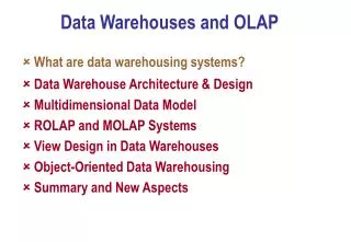
Data Warehouses • What is a data warehouse? • A multi-dimensional data model – data cube • Data warehouse architectures • Data warehouse implementation
What is Data Warehouse? • Defined in many different ways, but not rigorously. • A decision support database that is maintained separately from the organization’s operational database • Support information processing by providing a solid platform of consolidated, historical data for analysis. • Data warehousing: • The process of constructing and using data warehouses
Data Warehouse—Subject-Oriented • Organized around major subjects, such as customer, product, sales. • Focusing on the modeling and analysis of data for decision makers, not on daily operations or transaction processing. • Provide a simple and concise view around particular subject issues by excluding data that are not useful in the decision support process.
Data Warehouse—Time Variant • The time horizon for the data warehouse is significantly longer than that of operational systems. • Operational database: current value data. • Data warehouse data: provide information from a historical perspective (e.g., past 5-10 years) • Every key structure in the data warehouse • Contains an element of time, explicitly or implicitly • But the key of operational data may or may not contain “time element”.
Data Warehouse—Non-Volatile • A physically separate store of data transformed from the operational environment. • Operational update of data does not occur in the data warehouse environment. • Does not require transaction processing, recovery, and concurrency control mechanisms • Requires only two operations in data accessing: • initial loading of data and access of data.
Data Warehouse vs. Heterogeneous DBMS • Traditional heterogeneous DB integration: • Build wrappers/mediators on top of heterogeneous databases • Query driven approach • When a query is posed to a client site, a meta-dictionary is used to translate the query into queries appropriate for individual heterogeneous sites involved, and the results are integrated into a global answer set • Complex information filtering, compete for resources • Data warehouse: update-driven, high performance • Information from heterogeneous sources is integrated in advance and stored in warehouses for direct query and analysis
Why Separate Data Warehouse? • High performance for both systems • DBMS— tuned for OLTP: access methods, indexing, concurrency control, recovery • Warehouse—tuned for OLAP: complex OLAP queries, multidimensional view, consolidation. • A virtual DW (using views) may delay an OLTP machine
What is a data warehouse? • A multi-dimensional data model – data cube • Data warehouse architectures • Data warehouse implementation
D/W – OLAP (example) Problem: “is it true that shirts in large sizes sell better in dark colors?” sales ...
f size color color; size DataCubes ‘color’, ‘size’: DIMENSIONS ‘count’: MEASURE
DataCubes ‘color’, ‘size’: DIMENSIONS ‘count’: MEASURE f size color color; size
DataCubes ‘color’, ‘size’: DIMENSIONS ‘count’: MEASURE f size color color; size
DataCubes ‘color’, ‘size’: DIMENSIONS ‘count’: MEASURE f size color color; size
DataCubes ‘color’, ‘size’: DIMENSIONS ‘count’: MEASURE f size color color; size
DataCubes ‘color’, ‘size’: DIMENSIONS ‘count’: MEASURE f size color color; size DataCube
DataCubes SQL query to generate DataCube: • Naively (and painfully:) select size, color, count(*) from sales where p-id = ‘shirt’ group by size, color select size, count(*) from sales where p-id = ‘shirt’ group by size ...
DataCubes SQL query to generate DataCube: • with ‘cube by’ keyword: select size, color, count(*) from sales where p-id = ‘shirt’ cube by size, color
timeid locid sales pid Multidimensional Data Model • Collection of numeric measures, which depend on a set of dimensions. • E.g., measure Sales, dimensions Product(key: pid), Location (locid), and Time(timeid). 8 10 10 pid 11 12 13 30 20 50 25 8 15 locid 1 2 3 timeid
From Tables and Spreadsheets to Data Cubes • A data warehouse is based on a multidimensional data model which views data in the form of a data hyper-cube • A data cube, such as sales, allows data to be modeled and viewed in multiple dimensions • Dimension tables, such as item (item_name, brand, type), or time(day, week, month, quarter, year) • Fact table contains measures (such as dollars_sold) and keys to each of the related dimension tables • In data warehousing literature, an n-D base cube is called a base cuboid. The top most 0-D cuboid, which holds the highest-level of summarization, is called the apex cuboid. The lattice of cuboids forms a data cube.
Cube: A Lattice of Cuboids all 0-D(apex) cuboid time item location supplier 1-D cuboids time,item time,location item,location location,supplier 2-D cuboids time,supplier item,supplier time,location,supplier time,item,location 3-D cuboids item,location,supplier time,item,supplier 4-D(base) cuboid time, item, location, supplier
Conceptual Modeling of Data Warehouses • Modeling data warehouses: dimensions & measures • Star schema: A fact table in the middle connected to a set of dimension tables • Snowflake schema: A refinement of star schema where some dimensional hierarchy is normalized into a set of smaller dimension tables, forming a shape similar to snowflake • Fact constellations: Multiple fact tables share dimension tables, viewed as a collection of stars, therefore called galaxy schema or fact constellation
item time item_key item_name brand type supplier_type time_key day day_of_the_week month quarter year location branch location_key street city province_or_street country branch_key branch_name branch_type Example of Star Schema Sales Fact Table time_key item_key branch_key location_key units_sold dollars_sold avg_sales Measures
supplier item time item_key item_name brand type supplier_key supplier_key supplier_type time_key day day_of_the_week month quarter year city location branch city_key city province_or_street country location_key street city_key branch_key branch_name branch_type Example of Snowflake Schema Sales Fact Table time_key item_key branch_key location_key units_sold dollars_sold avg_sales Measures
item time item_key item_name brand type supplier_type time_key day day_of_the_week month quarter year location location_key street city province_or_street country shipper branch shipper_key shipper_name location_key shipper_type branch_key branch_name branch_type Example of Fact Constellation Shipping Fact Table time_key Sales Fact Table item_key time_key shipper_key item_key from_location branch_key to_location location_key dollars_cost units_sold units_shipped dollars_sold avg_sales Measures
Measures: Three Categories • distributive: if the result derived by applying the function to n aggregate values is the same as that derived by applying the function on all the data without partitioning. • E.g., count(), sum(), min(), max(). • algebraic:if it can be computed by an algebraic function with M arguments (where M is a bounded integer), each of which is obtained by applying a distributive aggregate function. • E.g.,avg(), min_N(), standard_deviation(). • holistic: if there is no constant bound on the storage size needed to describe a subaggregate. • E.g., median(), mode(), rank().
A Concept Hierarchy: Dimension (location) all all Europe ... North_America region Germany ... Spain Canada ... Mexico country Vancouver ... city Frankfurt ... Toronto L. Chan ... M. Wind office
Multidimensional Data • Sales volume as a function of product, month, and region Dimensions: Product, Location, Time Hierarchical summarization paths Region Industry Region Year Category Country Quarter Product City Month Week Office Day Product Month
Date 2Qtr 1Qtr sum 3Qtr 4Qtr TV Product U.S.A PC VCR sum Canada Country Mexico sum All, All, All A Sample Data Cube Total annual sales of TV in U.S.A.
Cuboids Corresponding to the Cube all 0-D(apex) cuboid country product date 1-D cuboids product,date product,country date, country 2-D cuboids 3-D(base) cuboid product, date, country
Typical OLAP Operations • Roll up (drill-up): summarize data • by climbing up hierarchy or by dimension reduction • Drill down (roll down): reverse of roll-up • from higher level summary to lower level summary or detailed data, or introducing new dimensions • Slice and dice: • project and select • Pivot (rotate): • reorient the cube, visualization, 3D to series of 2D planes. • Other operations • drill across: involving (across) more than one fact table • drill through: through the bottom level of the cube to its back-end relational tables (using SQL)
DataCubes Q: What operations should we support? Roll-up f size color color; size
DataCubes Q: What operations should we support? Drill-down f size color color; size
DataCubes Q: What operations should we support? Slice f size color color; size
DataCubes Q: What operations should we support? Dice f size color color; size
What is a data warehouse? • A multi-dimensional data model – data cube • Data warehouse architecture • Data warehouse implementation
Design of a Data Warehouse • Four views regarding the design of a data warehouse • Top-down view • allows selection of the relevant information necessary for the data warehouse • Data source view • exposes the information being captured, stored, and managed by operational systems • Data warehouse view • consists of fact tables and dimension tables • Business query view • sees the perspectives of data in the warehouse from the view of end-user
other sources Extract Transform Load Refresh Operational DBs Multi-Tiered Architecture Monitor & Integrator OLAP Server Metadata Analysis Query Reports Data mining Serve Data Warehouse Data Marts Data Sources Data Storage OLAP Engine Front-End Tools
OLAP Server Architectures • Relational OLAP (ROLAP) • Use relational or extended-relational DBMS to store and manage warehouse data and OLAP middle ware to support missing pieces • Include optimization of DBMS backend, implementation of aggregation navigation logic, and additional tools and services • greater scalability with increasing dimensionality • Multidimensional OLAP (MOLAP) • Array-based multidimensional storage engine; fast indexing to pre-computed summarized data • But in high-dimensionalities must be careful with sparseness • Hybrid OLAP (HOLAP) • detail data in ROLAP; summaries in MOLAP
What is a data warehouse? • A multi-dimensional data model – data cube • Data warehouse architecture • Data warehouse implementation
Efficient Data Cube Computation • Data cube can be viewed as a lattice of cuboids • The bottom-most cuboid is the base cuboid • The top-most cuboid (apex) contains only one cell • How many cuboids in an n-dimensional cube? • Materialization of data cube • Materialize every (cuboid) (full materialization), none (no materialization), or some (partial materialization) • Selection of which cuboids to materialize • Based on size, sharing, access frequency, etc.
Cube Computation: ROLAP-Based Method • Efficient cube computation methods • ROLAP-based cubing algorithms (Agarwal et al’96) • Array-based cubing algorithm (Zhao et al’97) • Bottom-up computation method (Bayer & Ramarkrishnan’99) • ROLAP-based cubing algorithms • Sorting, hashing, and grouping operations are applied to the dimension attributes in order to reorder and cluster related tuples • Grouping is performed on some subaggregates as a “partial grouping step” • Aggregates may be computed from previously computed aggregates, rather than from the base fact table
C c3 61 62 63 64 c2 45 46 47 48 c1 29 30 31 32 c 0 B 60 13 14 15 16 b3 44 28 56 9 b2 B 40 24 52 5 b1 36 20 1 2 3 4 b0 a0 a1 a2 a3 A Multi-way Array Aggregation for Cube Computation • Partition arrays into chunks (a small subcube which fits in memory). • Compressed sparse array addressing: (chunk_id, offset) • Compute aggregates in “multiway” by visiting cube cells in the order which minimizes the # of times to visit each cell, and reduces memory access and storage cost. What is the best traversing order to do multi-way aggregation?
C c3 61 62 63 64 c2 45 46 47 48 c1 29 30 31 32 c 0 B 60 13 14 15 16 b3 44 28 56 9 b2 40 24 52 5 b1 36 20 1 2 3 4 b0 a0 a1 a2 a3 A Multi-way Array Aggregation for Cube Computation B
Multi-way Array Aggregation for Cube Computation C c3 61 62 63 64 c2 45 46 47 48 c1 29 30 31 32 c 0 B 60 13 14 15 16 b3 44 28 B 56 9 b2 40 24 52 5 b1 36 20 1 2 3 4 b0 a0 a1 a2 a3 A
Multi-Way Array Aggregation for Cube Computation (Cont.) • Method: the planes should be sorted and computed according to their size in ascending order. • See the details of Example 2.12 (pp. 75-78) • Idea: keep the smallest plane in the main memory, fetch and compute only one chunk at a time for the largest plane • Limitation of the method: computing well only for a small number of dimensions • If there are a large number of dimensions, “bottom-up computation” and iceberg cube computation methods can be explored
Indexing OLAP Data: Bitmap Index • Index on a particular column • Each value in the column has a bit vector: bit-op is fast • The length of the bit vector: # of records in the base table • The i-th bit is set if the i-th row of the base table has the value for the indexed column • not suitable for high cardinality domains Base table Index on Region Index on Type
Indexing OLAP Data: Join Indices • Join index: JI(R-id, S-id) where R (R-id, …) S (S-id, …) • Traditional indices map the values to a list of record ids • It materializes relational join in JI file and speeds up relational join — a rather costly operation • In data warehouses, join index relates the values of the dimensions of a start schema to rows in the fact table. • E.g. fact table: Sales and two dimensions city and product • A join index on city maintains for each distinct city a list of R-IDs of the tuples recording the Sales in the city • Join indices can span multiple dimensions