Finding the Efficient Set (Chapter 5)
Finding the Efficient Set (Chapter 5). Feasible Portfolios Minimum Variance Set & the Efficient Set Minimum Variance Set Without Short-Selling Key Properties of the Minimum Variance Set Relationships Between Return, Beta, Standard Deviation, and the Correlation Coefficient.

Finding the Efficient Set (Chapter 5)
E N D
Presentation Transcript
Finding the Efficient Set(Chapter 5) • Feasible Portfolios • Minimum Variance Set & the Efficient Set • Minimum Variance Set Without Short-Selling • Key Properties of the Minimum Variance Set • Relationships Between Return, Beta, Standard Deviation, and the Correlation Coefficient
FEASIBLE PORTFOLIOS Expected Rate of Return (%) • When dealing with 3 or more securities, a complete mass of feasible portfolios may be generated by varying the weights of the securities: Stock 1 Portfolio of Stocks 1 & 2 Stock 2 Portfolio of Stocks 2 & 3 Stock 3 Standard Deviation of Returns (%)
Minimum Variance Set and theEfficient Set • Minimum Variance Set: Identifies those portfolios that have the lowest level of risk for a given expected rate of return. • Efficient Set: Identifies those portfolios that have the highest expected rate of return for a given level of risk.- Expected Rate of Return (%) Efficient Set (top half of the Minimum Variance Set) Minimum Variance Set MVP Note: MVP is the global minimum variance portfolio (one with the lowest level of risk) Standard Deviation of Returns (%)
Finding the Efficient Set • In practice, a computer is used to perform the numerous mathematical calculations required. To illustrate the process employed by the computer, discussion that follows focuses on: • 1. Weights in a three-stock portfolio, where: • Weight of Stock A = xA • Weight of Stock B = xB • Weight of Stock C =1 - xA - xB • and the sum of the weights equals 1.0 • 2. Iso-Expected Return Lines • 3. Iso-Variance Ellipses • 4. The Critical Line
Weights in a Three-Stock Portfolio(Data Below Pertains to the Graph That Follows) Invest in only one stock (Corners of the triangle) Invest in only two stocks (Perimeter of the triangle) Invest in all three stocks (Inside the triangle) Short-selling occurs when you are outside the triangle
Weights in a Three-Stock Portfolio (Continued)(Graph of Preceding Data) Weight of Stock B m h a f d g j k b Weight of Stock A c e l i n
Iso-Expected Return Lines • In the graph below, the iso-expected return line is a line on which all portfolios have the same expected return. • Given xA = weight of stock (A), and xB = weight of stock (B), the iso-expected return line is: xB = a0 + a1xA • Once a0 + a1 have been determined, we can solve for a value of xB and an implied value of xC, for any given value of xA
Iso-Expected Return Line(A graphical representation) Weight of Stock B xB = a0 + a1xA a0 = the intercept a1 = the slope Weight of Stock A Iso-Expected Return Line
Computing the Intercept and Slope of anIso-Expected Return Line
Iso-Expected Return Line for a Portfolio Return of 13% xB xA Iso-Expected Return Line For E(rp) = 13%
A Series of Iso-Expected Return Lines • By varying the value of portfolio expected return, E(rp), and repeating the process above many times, we could generate a series of iso-expected return lines. • Note: When E(rp) is changed, the intercept (a0) changes, but the slope (a1) remains unchanged. xB xA Series of Iso-Expected Return Lines in Percent 17 15 13 11
Iso-Variance Ellipse(A Set of Portfolios With Equal Variances) • First, note that the formula for portfolio variance can be rearranged algebraically in order to create the following quadratic equation:
Iso-Variance Ellipse (Continued) • Next, the equation can be simplified further by substituting the values for individual security variances and covariances into the formula.
Iso-Variance Ellipse (An Example) • Given the covariance matrix for Stocks A, B, and C: • Therefore, in terms of axB2 + bxB + c = 0 • Now, for a given 2(rp), we can create an iso-variance ellipse.
Generating the Iso-Variance Ellipse for aPortfolio Variance of .21 • 1. Select a value for xA • 2. Solve for the two values of xB • Review of Algebra: • 3. Repeat steps 1 and 2 many times for numerous values of xA
Generating the Iso-Variance Ellipse for aPortfolio Variance of .21 (Continued) • Example: xA = .5
Generating the Iso-Variance Ellipse for aPortfolio Variance of .21 (Continued) • A weight of .5 is simply one possible value for the weight of Stock (A). For numerous values of xA you could solve for the values of xB and plot the points in xB xA space: xB Iso-Variance Ellipse for 2(rp) = .21 .21 xA
Series of Iso-Variance Ellipses • By varying the value of portfolio variance and repeating the process many times, we could generate a series of iso-variance ellipses. These ellipses will converge on the MVP (the single portfolio with the lowest level of variance). xB .21 .19 .17 MVP xA
The Critical Line • Shows the portfolio weights for the portfolios in the minimum variance set. Points of tangency between the iso-expected return lines and the iso-variance ellipses. (Mathematically, these points of tangency occur when the 1st derivative of the iso-variance formula is equal to the 1st derivative of the iso-expected return line.) xB 16.9 15.6 13.6 9.4 7.4 6.1 .21 .17 .19 Critical Line MVP xA
Finding the Minimum Variance Portfolio (MVP) • Previously, we generated the following quadratic equation: • Rearranging, we can state: 1. Take the 1st derivative with respect to xB, and set it equal to 0: 2. Take the 1st derivative with respect to xA, and set it equal to 0: 3. Simultaneously solving the above two derivatives for xA & xB: xA = .06 xB = .58 xC = .36
Relationship Between the Critical Line and the Minimum Variance Set xB MVP C Critical Line * D xA
Relationship Between the Critical Line and the Minimum Variance Set (Continued) Expected Return C Minimum Variance Set MVP * D Standard Deviation of Returns
Minimum Variance Set When Short-Selling is Not Allowed (Critical Line Passes Through the Triangle) xB Critical Line Passes Through the Triangle MVP * xA
Minimum Variance Set When Short-Selling is Not Allowed (Critical Line Passes Through the Triangle)CONTINUED Expected Return With Short-Selling Stock (C) MVP * Without Short-Selling Stock (A) Standard Deviation of Returns
Minimum Variance Set When Short-Selling is Not Allowed (Critical Line Does Not Pass Through the Triangle) xB Critical Line Does NotPass Through the Triangle xA
Minimum Variance Set When Short-Selling is Not Allowed (Critical Line Does Not Pass Through the Triangle)CONTINUED Expected Return With Short-Selling Without Short Selling Standard Deviation of Returns
The Minimum Variance Set:(Property I) • If we combine two or more portfolios on the minimum variance set, we get another portfolio on the minimum variance set. • Example: Suppose you have $1,000 to invest. You sell portfolio (N) short $1,000 and invest the total $2,000 in portfolio (M). What are the security weights for your new portfolio (Z)? • Portfolio N: xA = -1.0, xB = 1.0, xC = 1.0 Portfolio M: xA = 1.0, xB = 0, xC = 0 Portfolio Z: xA = -1(-1.0) + 2(1.0) = 3.0 xB = -1(1.0) + 2(0) = -1.0 xC = -1(1.0) + 2(0) = -1.0
The Minimum Variance Set: (Property I)CONTINUED XB N M XA Z
The Minimum Variance Set:(Property II) • Given a population of securities, there will be a simple linear relationship between the beta factors of different securities and their expected (or average) returns if and only if the betas are computed using a minimum variance market index portfolio.
The Minimum Variance Set: (Property II)CONTINUED E(r) E(r) C M C M B B A A E(rZ) E(rZ) (r)
The Minimum Variance Set: (Property II)CONTINUED E(r) E(r) C C E(rZ) E(rZ) A A B B M M (r)
Notes on Property II • The intercept of a line drawn tangent to the bullet at the position of the market index portfolio indicates the return on a zero beta security or portfolio, E(rZ). • By definition, the beta of the market portfolio is equal to 1.0 (see the following graph). • Given E(rZ) and the fact that Z = 0, and E(rM) and the fact that M = 1.0, the linear relationship between return and beta can be determined.
Notes on Property IICONTINUED rM = M = 1.00 rM
Return, Beta, Standard Deviation, and the Correlation Coefficient • In the following graph, portfolios M, A, and B, all have the same return and the same beta. • Portfolios M, A, and B, have different standard deviations, however. The reason for this is that portfolios A and B are less than perfectly positively correlated with the market portfolio (M).
Return, Beta, Standard Deviation, and the Correlation Coefficient (Continued) E(r) E(r) j,M = 1.0 j,M = .7 M j,M = .5 M, A, B A B E(rZ) E(rZ) (r)
Return Versus Beta When the Market Portfolio (M**) is Inefficient E(r) E(r) C C M M** M** A A B B (r)