Enhanced CT Imaging Analysis: Speed and Accuracy through Unified LSU CT Techniques
This project aims to improve CT image analysis by testing the Unified LSU CT image method, which promises equal accuracy over traditional methods while enhancing speed. CT imaging utilizes density-based slices to visualize different tissues. Radiologists traditionally diagnose by identifying density abnormalities, a cumbersome process. Our ROC analysis using ROCKit software facilitates decision boundary determination in diagnostic imaging, optimizing sensitivity and specificity metrics. This study's outcomes could redefine imaging interpretation and foster more effective diagnostic processes.


Enhanced CT Imaging Analysis: Speed and Accuracy through Unified LSU CT Techniques
E N D
Presentation Transcript
What is a CT image? • CT= computed tomography • Examines a person in “slices” • Creates density-based images
Three different window densities • Bone- densest only bone shows detail, the rest is too dark to make out • Soft tissue- moderate density, bone is white, soft tissue is detailed, and “air space” is too dark • Lung- low density, bone and soft tissue white, and “air space” is detailed
How diagnoses are decided • Look for “abnormalities” in density
Our project- dare to compare • Test the new “unified LSU CT image”
Hypothesis • Unified LSU CT image: • Equally accurate • Faster
Methods • Our test • ROC Analysis • ROCKit Software
ROC Receiver Operating Characteristics Developed in 1950’s Statistical decision theory Used in business, economics, etc Goal: Is to be a meaningful tool for judging the performance of a diagnostic imaging system
Example • X Population y healthy z diseased • Gaussian distribution • Decision boundary • Interested in optimum decision boundary
EXAMPLE Non-diseased cases Diseased cases Threshold
EXAMPLE Non-diseased cases Diseased cases more typically:
DECISION BOUNDARY • TRUE NEGATIVE • TRUE POSITIVE • FALSE NEGATIVE • FALSE POSITIVE • What happens when you place the decision boundary?
DECISION BOUNDARY Non-diseased cases FALSE NEGATIVE IN RED Threshold Diseased cases TRUE POSITVE IN GREEN
DECISION BOUNDARY Non-diseased cases TRUE NEGATIVE IN WHITE Threshold Diseased cases FALSE POSITIVE IN WHITE
SENSITIVITY TPF Non-diseased cases SENSITIVITY = TP / TP + FN GREEN /GREEN+RED FNF = 1-TPF Threshold Diseased cases
SPECIFICITY TNF Non-diseased cases SPECIFICITY = TN / TN + FP LARGE WHITE / LARGE WHITE + SMALL WHITE FPF = 1-TNF Threshold Diseased cases
PREVALENCE • One of the important properties of ROC is that it is prevalence independent • Low prevalence is rare • Example • ROC IS NOT PREVALENCE DEPENDENT!
ROC CURVE Entire ROC curve TPF, sensitivity FPF, 1-specificity
ROC EXPERIMENT • Datasets • Two options • BINARY • MULT-SCALE RATING • Fitting curves
Rockit • Who developed Rockit? -Charles E. Metz @University of Chicago • What is Rockit? -curve fitting software calculates points for a Roc curve -calculates max probability of two Gaussian distributions • What is a Roc Curve? -describes how good the imaging systems is and accuracy of the given data and viewer’s results
Example 1 • 100 patients, 40 negative, 60 positive Given P P N P N N P… • Confidence Rating 1. Definitely Negative 2. Possibly Negative 3. Not sure 4. Possibly Positive 5. Definitely Positive This is the viewer’s results 5 4 2 4 1 2 3…. Now, from the confidence rating we consider 1=N and 2, 3, 4, 5=P to interpret view’s results. Interpretation of viewer’s result P P P P N P P… Comparing given data and interpretation TP TN FP FN 45 25 0 13 (a) TP- disease is present, diagnosed correctly (b) TN-disease is not present, diagnosed correctly (c) FP-person been diagnosed not having the disease, but the disease is present (d) FN-person been diagnosed having the disease, but the disease is not present. • Now, we compute the FPF and TPF. In order to compute the FPF, you need this formula FPF=1-TP/TP+FN and TPF=1-TN/TN+FP. • Therefore, in our case FPF=1-45/45+13= .224 and TPF=1-25/25+0=0 • So, our first point is (.224, 0).
Example 2 • Now we can compute a second point on the Roc curve. • We consider a different confidence rating. • 1, 2=N and 3, 4, 5=P Results based on viewer’s answer from above P P N P N N N N…. • The new Truth table is: TP TN FP FN 46 28 0 15 • Now the FPF=1-46 / 46+15 =.245 and TPF= 1-28/ 28+0 = 0 • Now, we have our second point (.245, 0) • Based upon the viewer’s results, a third and forth point can be created by changing the confidence ratings. 1, 2, 3=N and 4, 5=P ->third point 1, 2, 3, 4=N and 5=P ->forth point • Therefore, five confidence ratings give you four points on the Roc curve.
Rockit input • For Condition 1: d Enter the Total Number of Actually-Negative Cases (an integer): 40 Beginning with category 1 and separated by blanks, Enter (on one line, integers only) the number of responses to Actually- Negative cases in each category: 1 2 3 4 5 23 10 2 3 2 • For Condition 1: d Enter the Total Number of Actually-Positive Cases (an integer): 60 Beginning with category 1 and separated by blanks, Enter (on one line, integers only) the number of responses to Actually- Positive cases in each category: 1 2 3 4 5 2 2 3 10 43
Rockit • a, b parameters - a represents separation of the Gaussian distributions -b represents width of two Gaussian distributions • Open excel template to enter a, b parameters • Roc curve is produced