Sample CT Image
Sample CT Image. X-ray. 2 % attenuation change detectable in film. CT. 0.2 % change in attenuation coefficient. y. x. f(x,y). CT, like X-ray measure line integrals. ∑ ∑ ∑ ∑ ∑. g(R) = CT detector array output. g(R). Direct Methods. Radon Transform 1917

Sample CT Image
E N D
Presentation Transcript
X-ray 2 % attenuation change detectable in film CT 0.2 % change in attenuation coefficient y x f(x,y) CT, like X-ray measure line integrals ∑ ∑ ∑ ∑ ∑ g(R) = CT detector array output g(R)
Direct Methods Radon Transform 1917 Central Section Theorem - Bracewell The transform of each projection forms a line, at that angle, in the 2D FT of f(x,y) g(R) = ∫ f(x,y) dy f(x,y) We will skip the Algebraic Reconstruction Technique g(R)
First, let’s think of our experience on the meaning of F(u,0) in the Fourier transform. v F(u,0) u {f(x,y)} => F (u,v) = ∫∫ f(x,y) e -i 2π (ux +vy) dx dy F(u,0) = ∫ [ ∫ f(x,y) dy] e -i 2π ux dx So F(u,0) is the Fourier transform of the projection formed from line integrals along the y direction.
Computed Tomography • Uses a collimator to keep exposure to a slice • Builds image from multiple projections • We will assume parallel rays for now. • Actually how first generation scanners worked. • Translate source and single detector across body for one angle • Then rotate source and detector to get next angle
Central Section Theorem The 1D Fourier Transform of a projection at angle forms a line in the 2D Fourier space of the image at the same angle. y Incident X-rays R ø x R r f(x,y) Detected g (R)
Incident x-rays pass through the object f(x,y) from upper left to lower right at the angle 90 + . For each point R, a different line integral describes the result on the function g (R). g (R) is measured by an array of detectors or a moving detector. The thick line is described by x cos + y sin = R I have just drawn one thick line to show one line integral, but the diagram is general and pertains to any value of R.
The projection g (R) can thus be calculated as a set of line integrals, each at a unique R. g (R) = ∫ ∫ f(x,y) (x cos + y sin - R) dx dy 2π ∞ g (R) = ∫ ∫ f(r, f) (r cos ( - f ) - R) r dr df 0 0 In the second equation, we have translated to polar coordinates. Again g (R) is a 1D function of R.
Let’s consider the 2D FFT F(u,v) = ∫ ∫ f(x,y) e -i 2π (ux + vy) dx dy In polar coordinates, u = cos v = sin F(,) = ∫ ∫ f(x,y) exp [ -i 2π (x cos + y sin )]dx dy When x cos + y sin = constant, exp [ -i 2π (x cos + y sin )] is a linear phase shift. This is the Fourier transform of a shifted delta function. Let’s let the constant = R and write the complex exponential as the FT of a function. F(,) = ∫y ∫ xf(x,y) F[( x cos + y sin - R)] dx dy F(,) = ∫y ∫x f(x,y) [∫ [( x cos + y sin - R)] e-i 2π rR dR] dx dy
F(,) = ∫ ∫ f(x,y) [∫ [( x cos + y sin - R)] e-i 2π rR dR] dx dy Recall how we wrote the projection as a double integral of f(x,y) where a delta function performs the line integral, g (R) = ∫ ∫ f(x,y) (x cos + y sin - R) dx dy We take the Fourier Transform of g (R): F{g (R)}= ∫R [ ∫y ∫x f(x,y) ( x cos + y sin - R) dx dy] e-i 2πrR dR dxdy which is exactly what we wrote for F(r, ) above! Thus, F{g (R)} = F(r, )
Central Section OrProjection Slice Theorem F{g (R)} = F(r, ) So in words, the Fourier transform of a projection at angle gives us a line in the polar Fourier space at the same angle .
BATTLESHIP Battleship: New Rules Old way EW 2/ NS 3 Hit! EW 5/ NS 6 Miss! North/South Data East - West Data
BATTLESHIP Battleship: New Rules Tell the other player how many times you see a battleship in a square along each column. I started it for you. Finish up the other gray squares on the bottom row. North/South Data East - West Data
BATTLESHIP Battleship: New Rules Here it is finished. North/South Data East - West Data
BATTLESHIP If this is all your opponent told you, could you find where the battleships were? North/South Data East - West Data
BATTLESHIP Battleship: New Rules What if your opponent also had to tell you the number of ships in squares along each row? Complete the gray squares on the right side. I started it for you. North/South Data East - West Data
BATTLESHIP North/South Data Here are all the answers. East - West Data
BATTLESHIP North/South Data Can you find the ships now if you just knew the gray squares? One idea: Smear the East West numbers all the way up the columns. This tells us that we should not spend much time looking along EW4 or EW9. But there is something probably up in EW8 East - West Data
BATTLESHIP Next, smear the North/ South numbers to the left and add them to what was in the grid before. Where do you think the ships are? By the biggest numbers? Is this always true? Let’s see. North/South Data East - West Data
BATTLESHIP North/South Data Here I finished smearing the north/south numbers to the left and adding them to the east/west numbers. Where do you think the ships are? By the biggest numbers? Is this always true? Let’s see. East - West Data
BATTLESHIP North/South Data Next, smear the North/ South numbers to the left and add them to what was in the grid before. Are the battleships where the biggest numbers are? All of the time? Some of the time? East - West Data
BATTLESHIP What if we can measure along the diagonals? 0 0 1 1 1 0 0 1 1 1 2 1 1 0 0 0 0
BATTLESHIP Now add the diagonal information to our totals. Are we doing any better? Are the battleships where the biggest numbers are more often?
Reconstruction from Projections Crude Idea 1: Take each projection and smear it back along the lines of integration it was calculated over. Result from a back projection: b (x,y) = ∫ g (R) (x cos + y sin - R) dR Adding up all the back projections from all the angles gives, fback-projected (x,y) = ∫ b (x,y) d π ∞ fb (x,y) = ∫ d ∫ g (R) (x cos + y sin - R) dR 0 -∞
Let’s calculate an impulse response to see how the reconstruction does. g (R) = (R) That is, (x,y) causes a (R) projection. By calculating the back- projected image, fb (x,y), we will be calculating the impulse response. hb (x,y) = fb (x,y) for this delta object Recall x cos + y sin - R = r cos ( - f) - R hb (r,) = ∫ d ∫ (R) (r cos ( - f ) - R) dR We can simplify the integration over R by realizing that the first delta function will be non-zero only when R=0. Then we will only have one integral across π = ∫ (r cos ( - f)) d 0
Now [f(x)] = ∑ (x - xn) / |f’(xn)| n Only one root (zero) in range of integral cos ( - f) = 0 - f = π/2 = π/2 + f Since denominator has to be evaluated at = π/2 + f
Back-projected impulse response hb(r) = 1/r fb (x,y) = f(x,y) ** 1/r Fb (,) = F (,) / since F{1/r}= 1/
Back projected image is blurred by convolution with 1/r Where intuitively does the 1/r come from? We must account for this blurring to properly reconstruct the image. How does 1/r convolution look in image space? In frequency space?
Low spatial frequency data is overweighted. Filter to compensate for this. Weighted by 1/. • Solution - filter each projection by || to account for the uneven sampling density • Steps: • Calculate projection • Transform projection • Weight with || • Inverse transform • Back project • Add all angles Mathematically, ∫ d ∫ F -1 { F{g (R)} || } (x cos + y sin - R) dR Solution
Filtered Back-Projection The reconstruction described is known as filtered back-projection. What is downside of the described filter, || ?
Filtered Back-Projection What is downside of this filter? Band limit filter to: 0 Filter rect ( / 20) c(R) = ?
Convolution Back Projection Instead of converting to frequency domain, use convolution in the image domain π ∞ ∫ d ∫ [ g (R) * c (R) ] ( x cos + y sin - R) dR 0 -∞ Each projection is convolved with c (R) and then back projected. Describe c (R) C (p) = | | c (R) = lim 2 (2 - 4π2R2) / (2 + 4π2R2)2 0
Better Design 1.0 - 0 0 c (R) = 0 [ 2 sinc (2 0 R) - sinc 2 (0 R)] Actual Filters : Ram-Lak : Shepp-Logan
a) Ramachandran-Lakshminarayanan kernel b) Shepp-Logan kernel. Solid lines represent h() and circles hk c) Representation of the filter functions corresponding to hR and hS


![[ Sample Image: Place a 9.5” x 4.75” image here ]](https://cdn2.slideserve.com/3757091/slide1-dt.jpg)