En tropy as Computational Complexity Computer Science Replugged
240 likes | 366 Vues
This paper explores how to estimate the additional time required to fully solve a problem that has been partially addressed. Utilizing concepts from computational complexity and entropy, we analyze various scenarios, including the recovery of data after power interruption. By understanding the relationship between time and entropy via Shannon's information theory, we assess the efficiency of algorithms like minimal mergesort and minimum spanning trees. We present significant theorems that link the detailed characteristics of problem states and their respective time complexities.

En tropy as Computational Complexity Computer Science Replugged
E N D
Presentation Transcript
Entropy as Computational ComplexityComputer Science Replugged Tadao Takaoka Department of Computer Science University of Canterbury Christchurch, New Zealand
Genera framework and motivation • If the given problem is partially solved, how much more time is needed to solve the problem completely. Time =Time spent + Time to be spent Output Input data Algorithm Save Recover Saved data A possible scenario: Suppose computer is stopped by power cut and partially solved data are saved by battery. After a while power is back on , data are recovered, and computation resumes. How much more time ? Estimate from the partially solved data.
Entropy • Thermodynamics kloge(Q), Q number of states in the closed system, k Boltzman constant • Shannon’s information theory –[i=1, n] pilog(pi), where n=26 for English • Our entropy, algorithmic entropy to describe computational complexity
Definition of entropy • Let X be the data set and X be decomposed like S(X)=(X1, …, Xk). Each Xi is solved. S(X) is a state of data, and abbreviated as S. Let pi=|Xi|/|X|, and |X|=n. The entropy H(S) is defined by • H(S) =[i=1, k]|Xi|log(|X|/|Xi|)=-n[i=1,k]pilog(pi) • pi = 1,0 H(S) nlog(k), maximum when all |Xi| are equal to 1/k.
Amortized analysis • The accounting equation at the i-th operation becomes • ai = ti - ΔH(Si), actual time – decrease of entropy where ΔH(Si) = H(Si-1) - H(Si). • Let T and A be the actual total time and the amortized total time. • Summing up ai for i=1, ..., N, we have • A = T + H(SN) - H(S0), • or T = A + H(S0) - H(SN). • In many applications, A=0 and H(SN)=0, meaning T=H(S0) • For some applications, ai = ti - cΔH(Si) for some constant c
Problems analyzed by entropy • Minimal Mergesort : merging shortest ascending runs • Shortest Path Problem: Solid parts solved. Make a single shortest path spanning tree • Minimum Spanning Tree : solid part solved. Make a single tree souurce
Three examples with k=3 • (1) Minimal mergesort Time =O(H(S)) • Xi are ascending runs • S(X) = (2 5 6 1 4 7 3 8 9) • X1=(2 5 6), X2 =(1 4 7), X3=(3 8 9) • (2) Shortest paths for nearly acyclic graphs Time=O(m+H(S)) • G=(V, E) is a graph. S(V)=(V1, V2, V3) • Vi is an acyclic graph dominated by vi • (3) Minimum spanning tree Time = O(m+H(S)) • S(V)=(V1, V2, V3), subgraph Gi=(Vi, Ei) is the induced graph from Vi. We assume minimum spanning tree Ti for Gi is already obtained
Time complexities of the three problems • Minimal mergesort O(H(S)) • worst case O(nlog(n)) • Single source shortest paths O(m+H(S)) • worst case time O(m+nlog(n)) • data structures: Fibonacci heap or 2-3 heap • Minimum cost spanning trees O(m+H(S)) • Presort of edges (mlog(n)) excluded • worst case time O(m+nlog(n))
Which is more sorted? Entropy H(S) = nlog(k), k=4 Entropy H(S) = O(n), more sorted
Minimal mergesort picture • Metasort S(X) S’(X) M L ... . . . W1 W2 merge W
Minimal MergesortM L : first list of L is moved to the last of M • Meta-sort S(X) into S’(X) by length of Xi • Let L = S’(X); /* L : list of lists */ • M=φ; M L; /* M : list of lists */ • If L is not empty, M L; • for i=1 to k-1 do begin • W1 M; W2 M; • W=merge(W1, W2); • While L φ and |W|>first(L) do M L • M L • End
Merge algorithm for lists of lengths m and n (m ≦ n)in time O(mlog(1+n/m)) by Brown and Tarjan • Lemma. Amortized time for i-th merge ai≦0 • Proof. Let |W1|=n1 and |W2|=n2 • ΔH = n1log(n/n1)+n2log(n/n2)-(n1+n2)log(n/(n1+n2) • = n1log(1+n2/n1)+n2log(1+n1/n2) • ti≦ O(n1log(1+n2/n1)+n2(log(1+n1/n2)) • ai = ti – cΔH ≦0
Main results in minimal mergesort • Theorem. Minimal mergesort sorts sequence S(X) in O(H(S)) time • If pre-scanning is included, O(n+H(S)) • Theorem. Any sorting algorithm takes • (H(S)) time if |Xi| 2 for all i. • If |Xi|=1 for all i, S(X) is reverse-sorted, and it can be sorted in ascending order, in O(n) time.
Minimum spanning trees • Blue fonts : vertices 1 8 7 5 9 3 8 2 2 T3 5 10 3 4 3 4 4 4 T1 2 2 11 6 1 9 6 7 5 T2 L=(1 2 2 2 3 3 4 4 4 5 5 6 7 8 9) L=(4 5 5 6 7 8 9) name =(1 1 1 1 2 2 2 3 3 3 3) (1 1 1 1 1 1 1 3 3 3 3)
Kruskal’s completion algorithm • 1 Let the sorted edge list L be partially scanned • 2 Minimum spanning trees for G1, ..., Gk have been obtained • 3 for i=1 to k do for v in Vkdo name[v]:=k • 4 while k > 1 do begin • 5Remove the first edge (u, v) from L • 6 if u and v belong to different sub-trees T1and T2 • 7 then begin • 8Connect T1 and T2 by (u, v) • 9 Change the names of the nodes in the smaller tree • to that of the larger tree; • 10k:=k - 1; • 11 end • 12 end.
Entropy analysis for name changes • the decrease of entropy is • ΔH = n1log(n/n1) + n2log(n/n2) • -(n1+n2)log(n/(n1+n2)) • = n1log(1+n2/n1) + n2log(1+n1/n2) • ≥ min{n1, n2} • Noting that ti <= min{n1, n2}, amortized time becomes • ai = ti - ΔH(Si) ≦ 0 • Scanning L takes O(m) time. Thus • T=(m+H(S0)), where H(S0) is the initial entropy.
Single source shortest pathsExpansion of solution set • S: solution set of vertices to which shortest distances are known • F: frontier set of vertices connected from solution set by single edges Time = O(m + nlogn) S : solution set F : frontier w s w v
Priority queueF is maintained in Fibonacci or 2-3 heap Delete-min O(log n) Decrease key O(1) Insert O(1)
Dijkstra’s algorithm for shortest paths with a priority queue, heap with time= O(m+nlog(n)) • d[s]=0; • S={s}; F={w|(s,w) in out(s)}; d[v]=c[s,v] for all v in F; • while |S|<n do • delete v from F such that d[v] is minimum //delete-min • add v to S O(log n) • for w in out(v) do • if w is not in S then • if w is if F then d[w]=min{d[v], d[v]+c[v,w] //decrease-key • O(1) • else {d[w]=d[v]+c[v,w]; add w to F} //insert O(1) • end do
Sweeping algorithm • Let v1, …, vn be topologically sorted • d[v1]=0; • for i=2 to n do d[vi]= • for i=1 to n do do • for w in out(vi) do • d[w]=min{d[vi], d[vi]+c[vi,w]} • Time = O(m)
Efficient shortest path algorithm for nearly acyclic graphs • d[s]=0 • S={s}; F={w|(s,w) in out(s)}; // F is organized as priority queue • while |S|<n do • if there is a vertex in F with no incoming edge from V-S • then choose v // easy vertex O(1) • else choose v from F such that d[v] is minimum //difficult O(log n) • add v to S find-min • Delete v from F // delete • for w in out(v) do • if w is not in S then • if w is in F then d[w]=min{d[v], d[v]+c[v,w] //decrease-key • else {d[w]=d[v]+c[v,w]; add w to F} //insert O(1) • end do
Easy vertices and difficult vertices F S w s w difficult v easy
Nearly acyclic graph • Acyclic components are regarded assolved There are three acyclic components in this graph. Vertices in the component Vi can be deleted from the queue once the distance to the trigger vi is finalized ui Vi Acyclic graph topologically sorted 7 1 3 2 8
Entropy analysis of the shortest path algorithm • Generalization delete-min = (find-min, delete) • to (find-min, delete, …, delete) • There are t difficult vertices u1, …, ut. • Each ui and the following easy vertices form an acyclic sub-graph. Let {v1,…, vk}, where v1=ui for some i, be one of the roots of the above acyclic sub-graphs. Let the number of descendants of vi in the heap be ni. • Delete v1, …, vk. Time = log(n1)+…+log(nk) ≦O(klog(n/k). • Let us index k by i for ui. Then the total time for deletes is O(k1log(n/k1)+…+ktlog(n/kt) = O(H(S)) where S(V)=(V1, …, Vt). Time O(tlog n) for t find-mins is absorbed in O(H(S)) • The rest of the time is O(m). Thus total time is O(m+O(H(S))