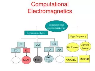
Computational Electromagnetics
computational electromagnetics. rigorous methods. High frequency. DE. current based. IE. VM. field based. TD. FD. TD. FD. PO/PTD. FDTD TLM. FEM. MoM. GO/GTD. Computational Electromagnetics. Computational Electromagnetics.

Computational Electromagnetics
E N D
Presentation Transcript
computational electromagnetics rigorous methods High frequency DE current based IE VM field based TD FD TD FD PO/PTD FDTD TLM FEM MoM GO/GTD Computational Electromagnetics
Computational Electromagnetics Electromagnetic problems are mostly described by three methods: Differential Equations (DE) Finite difference (FD, FDTD) Integral Equations (IE) Method of Moments (MoM) Minimization of a functional (VM) Finite Element (FEM) Theoretical effort less more Computational effort more less
Conventional Calculus The operation of diff. of a function is a well-defined procedure The operations highly depend on the form of the function involved Many different types of rules are needed for different functions For some complex function it can be very difficult to find closed form solutions Numerical differentiation Is a technique for approximating the derivative of functions by employing only arithmetic operations (e.g., addition, subtraction, multiplication, and division) Commonly known as “finite differences” Introduction to differentiation
y f(x) xi x f(xi) Taylor Series Problem: For a smooth function f(x), Given: Values of f(xi) and its derivatives at xi Find out: Value of f(x) in terms of f(xi), f(xi), f(xi), ….
Taylor’s Theorem If the function f and its n+1 derivatives are continuous on an interval containing xiand x, then the value of the function f at x is given by
Finite Difference Approximationsof the First Derivative using the Taylor Series (forward difference) Assume we can expand a function f(x) into a Taylor Series about the point xi+1 y f(x) h xi xi+1 x f(xi) f(xi+1) h
Finite Difference Approximationsof the First Derivative using the Taylor Series (forward difference) Assume we can expand a function f(x) into a Taylor Series about the point xi+1 Ignore all of these terms
Finite Difference Approximationsof the First Derivative using the Taylor Series (forward difference) y f(x) h xi xi+1 x f(xi) f(xi+1)
Finite Difference Approximationsof the First Derivative using the forward difference: What is the error? The first term we ignored is of power h1. This is defined as first order accurate. First forward difference
Finite Difference Approximationsof the First Derivative using the Taylor Series (backward difference) Assume we can expand a function f(x) into a Taylor Series about the point xi-1 y f(x) h xi-1 xi x f(xi-1) f(xi) -h
Finite Difference Approximationsof the First Derivative using the Taylor Series (backward difference) Ignore all of these terms First backward difference
Finite Difference Approximationsof the First Derivative using the Taylor Series (backward difference) y f(x) h xi-1 xi x f(xi-1) f(xi)
Finite Difference Approximationsof the Second Derivative using the Taylor Series (forward difference) y f(x) h xi+2 xi xi+1 x f(xi) f(xi+2) f(xi+1) (1) (2) (2)-2* (1)
Finite Difference Approximationsof the Second Derivative using the Taylor Series (forward difference) y f(x) h xi+2 xi xi+1 x f(xi) f(xi+2) f(xi+1) Recursive formula for any order derivative
Centered Difference Approximation (1) (2) (1)-(2)
Finite Difference Approximationsof the First Derivative using the Taylor Series (central difference) y f(x) h xi-1 xi xi+1 x f(xi-1) f(xi+1) f(xi)
Second Derivative Centered Difference Approximation (central difference) (1) (2) (1)+(2)
Using Taylor Series Expansions we found the following finite-differences equations FORWARD DIFFERENCE BACKWARD DIFFERENCE CENTRAL DIFFERENCE CENTRAL DIFFERENCE
Finite Difference Approx. Partial Derivatives Problem: Given a function u(x,y) of two independent variables how do we determine the derivative numerically (or more precisely PARTIAL DERIVATIVES) of u(x,y)
STEP #1: Discretize (or sample) U(x,y) on a 2D grid of evenly spaced points in the x-y plane Pretty much the same way
2D GRID u(xi-1,yj+1) u(xi,yj+1) u(xi+1,yj+1) u(xi+2,yj+1) y axis yj+1 u(xi,yj) u(xi+1,yj) u(xi+2,yj) u(xi-1,yj) yj u(xi-1,yj-1) u(xi,yj-1) u(xi+1,yj-1) u(xi+2,yj-1) yj-1 u(xi-1,yj-2) u(xi,yj-2) u(xi+1,yj-2) u(xi+2,yj-2) yj-2 xi-1 xi xi+1 xi+2 x axis
ui,j+1 y axis j+1 ui-1,j ui,j ui+1,j j ui,j-1 j-1 j-2 i-1 i i+1 i+2 SHORT HAND NOTATION x axis
Partial First Derivatives Problem: FIND recall:
Partial First Derivatives Problem: FIND Dy These are central difference formulas Are these the only formulas we could use? Could we use forward or backward difference formulas? Dx
Partial First Derivatives: short hand notation Problem: FIND Dy Dx
Partial Second Derivatives Problem: FIND recall:
Partial Second Derivatives Problem: FIND Dy Dx
Partial Second Derivatives: short hand notation Problem: FIND Dy Dx
FINITE DIFFERENCE ELECTROSTATICS Electrostatics deals with voltages and charges that do no vary as a function of time. Poisson’s equation Laplace’s equation Where, F is the electrical potential (voltage), r is the charge density and e is the permittivity.
F3 Fo F2 F1 FINITE DIFFERENCE ELECTROSTATICS: Example Find F(x,y) inside the box due to the voltages applied to its boundary. Then find the electric field strength in the box.
Electrostatic Example using FD Problem: FIND Dy Dx
Electrostatic Example using FD Problem: FIND If Dx = Dy
Electrostatic Example using FD Problem: FIND • Iterative solution technique: • Discretize domain into a grid of points • Set boundary values to the fixed boundary values • Set all interior nodes to some initial value (guess at it!) • Solve the FD equation at all interior nodes • Go back to step #4 until the solution stops changing • DONE
Electrostatic Example using FD MATLAB CODE EXAMPLE
F=0 F=0 F=0 F=0 FINITE DIFFERENCE Waveguide TM modes: Example Where for TM modes and If then kz becomes imaginary and the mode does not propagate.
F=0 F=0 F=0 F=0 FINITE DIFFERENCE Waveguide TM modes: Example Goal: Find all permissible values of kt and the corresponding mode shape (F(x,y)) for that mode.
Waveguide Example using FD Problem: FIND Dy Dx
Waveguide Example using FD Problem: FIND If Dx = Dy=h
F=0 F=0 F=0 F=0 Waveguide Example using FD let where N is the number of interior nodes (i.e. not on a boundary) If we now apply the FD equation at all interior nodes we can form a matrix equation Where I is the identity matrix
Waveguide Example using FD is an eigenvalue equation usually cast in the form The eigenvalues will provide the permissible values for the transverse wavenumber kt and the eigenvectors are the corresponding mode shapes (F(x,y))
F=0 F=0 F3 F4 F=0 F=0 W F1 F2 F=0 F=0 h F=0 F=0 W Waveguide Example using FD
F=0 F=0 F3 F4 F=0 F=0 W F1 F2 F=0 F=0 h F=0 F=0 W Waveguide Example using FD Node #1: Node #2: Node #3: Node #4: Solve using the Matlab “eig” function
Waveguide Example using FD is an eigenvalue equation usually cast in the form The eigenvalues will provide the permissible values for the transverse wavenumber kt and the eigenvectors are the corresponding mode shapes (F(x,y)) HOMEWORK: WRITE A MATLAB PROGRAM THAT CALCULATES THE TRANSVERSE WAVENUMBERS AND MODE SHAPES FOR A RECTANGULAR WAVEGUIDE FOR TM MODES
Some big advantages • Broadband response with a single excitation. • 3D models easily. • Frequency dependent materials accommodated. • Most parameters can be generated e.g. • Scattered fields • antenna patters • RCS • S-parameters • etc…..