Univariate Descriptive Statistics
Univariate Descriptive Statistics. Chapter 2. Lecture Overview. Tabular and Graphical Techniques Distributions Measures of Central Tendency Measures of Dispersion. Tabular and Graphical Techniques. Frequency Tables Ungrouped Grouped Histograms Cumulative Frequency Histogram.

Univariate Descriptive Statistics
E N D
Presentation Transcript
Univariate Descriptive Statistics Chapter 2
Lecture Overview • Tabular and Graphical Techniques • Distributions • Measures of Central Tendency • Measures of Dispersion
Tabular and Graphical Techniques • Frequency Tables • Ungrouped • Grouped • Histograms • Cumulative Frequency Histogram
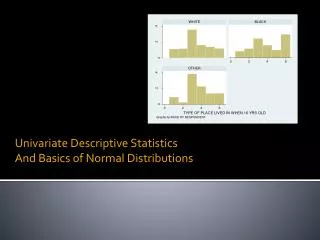
Histograms Note: sometimes percent is on the Y axis rather than frequency
Key Concepts • Choosing Intervals (i.e., choosing your “bins”) • Rules from the textbook (pages 38 – 39) • Commonly Used Examples from GIS • Equal Interval • Quantiles (e.g., quartiles and quintiles) • Natural Breaks • Standard Deviation
Rules For Bin Sizes • Note: This is very relevant for GIS • Rule 1: Use intervals with simple bounds • Rule 2: Respect natural breakpoints • Rule 3: Intervals should not overlap • Rule 4: Intervals should be the same width • Rule 5: Select an appropriate number of classes
The Effect of Classification • Equal Interval • Splits data into user-specified number of classes of equal width • Each class has a different number of observations
The Effect of Classification • Quantiles • Data divided so that there are an equal number of observations are in each class • Some classes can have quite narrow intervals
The Effect of Classification • Natural Breaks • Splits data into classes based on natural breaks represented in the data histogram
The Effect of Classification • Standard Deviation • Mean + or – Std. Deviation(s)
Key Concepts • Making sense of your histograms using distributions • Rectangular • Unimodal • Bimodal • Multimodal • Skew (positive and negative)
Skew • An asymmetrical distribution
Measures of Central Tendency • Measures of central tendency • Measures of the location of the middle or the center of a distribution • Mean, median, mode, midrange
Definitions • Midrange • Mode • Median • Quantiles • Mean
Definitions • Sample Mean • Population Mean
Description of Mean • Mean – Most commonly used measure of central tendency • Average of all observations • The sum of all the scores divided by the number of scores • Note: Assuming that each observation is equally significant
Symbols • n : the number of observations • N : the number of elements in the whole population • Σ : this (capital sigma) is the symbol for sum • i : the starting point of a series of numbers • X: one element in our dataset, usually has a subscript (e.g., i, min, max) • : the sample mean • : the population mean
Summation Notation: Components refers to where the sum of terms ends indicates what we are summing up indicates we are taking a sum refers to where the sum of terms begins
Mathematical Notation of Mean • The mathematical notation used most often in this course is the summation notation • The Greek letter capital sigma is used as a shorthand way of indicating that a sum is to be taken: The expression is equivalent to:
Summation Notation: Simplification • A summation will often be written leaving out the upper and/or lower limits of the summation, assuming that all of the terms available are to be summed
Equation for Mean Sample mean: Population mean:
Example Mean Calculations • Example I • Data: 8, 4, 2, 6, 10 • Example II • Sample: 10 trees randomly selected from Battle Park • Diameter (inches): 9.8, 10.2, 10.1, 14.5, 17.5, 13.9, 20.0, 15.5, 7.8, 24.5
Example Mean Calculations • Example III Annual mean temperature (°F) Monthly mean temperature (°F) at Chapel Hill, NC (2001).
Examples IV & V Mean annual precipitation (mm) Mean 1198.10 (mm) Mean annual temperature (°F) Mean 58.51 (°F) Chapel Hill, NC (1972-2001)
Explanation of Mean • Advantage • Sensitive to any change in the value of any observation • Disadvantage • Very sensitive to outliers Mean = 6.19 m without #8 Mean = 8.10 m with #8
Measures of Dispersion • Used to describe the data dispersion/spread/variation/deviation numerically • Usually used in conjunction with measures of central tendency
Measures of variation # of obs score score Low variation High variation Groups have equal means and equal n, but one varies more than the other
Definitions • Range • Mean Deviation • Variance • Standard Deviation • Coefficient of Variation • Pearson’s
Symbols • s2 : the sample variance • σ2 : the population variance • s : the sample standard deviation • σ : the population standard deviation
Sample Variance and Standard Deviation Variance Standard Deviation Note: as with the mean there are both sample and population standard deviations & variances
Next Class • Read chapter 3 • Work on the homework • Come with questions • Bring your laptop