A numerical study of the interaction of the convective boundary layer and orographic

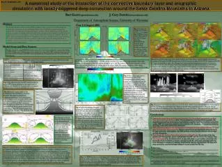
1. P5-27: EMS2010-239 A numerical study of the interaction of the convective boundary layer and orographic circulation with locally-triggered deep convection around the Santa Catalina Mountains in Arizona Bart Geerts (geerts@uwyo.edu) J. Cory Demko (coryuw@uwyo.edu) Department of Atmospheric Science, University of Wyoming Abstract Case 1: 6 August 2006 The Weather, Research, and Forecasting (WRF) modeling system is used for several IOPs during the Cumulus Photogrammetric, In situ and Doppler Observations (CuPIDO) campaign, conducted in summer 2006 around the Santa Catalina Mountains in southeast Arizona (Damiani et al. 2008), with the purpose to examine the interplay between boundary-layer convergence and orographic thunderstorms in a weakly-sheared environment subject to strong surface heating. This study builds on Demko and Geerts (2010), which examines thermally-forced orographic boundary-layer circulations without deep convection. The study is motivated by the fact that operational models poorly capture the timing and intensity of orographic convection, mostly due to inaccurate coupling between boundary-layer processes and cumulus convection over complex terrain. Fig. 4: North-south average cross section of θ’west,east, u’, w,and PBL height for 12 (a), 15 (b), 18 (c), and 21 (d) UTC 06 August 2006. The perturbations are from the mean profiles. These profiles are shown on the side: θwest (solid), θeast (dashed) (profiles on the left) and u (profile on the right). Model Setup and Data Sources Detailed simulations using WRF-NMM model version 3.0.1.1 have been conducted on several days during CuPIDO. Model output validation data sources used in this study include ISFF stations located around the mountain, KTUS soundings, and WRF output, specifically the 24 hr period from 06 UTC to 06 UTC the following day. Fig. 8: 2 m potential temperature (color shaded surface), 10 m wind (barbs), and cloud liquid or frozen water isosurface of 0.01 gkm-1 for WRF forecast hours 19, 20, 21 (top/left to right), 22, 23 UTC 06 August, and 00 UTC 07 August (bottom/left to right). Also illustrated are 1 hr accumulated precipitation contours over terrain in intervals of 0.01, 0.1, 0.25, 0.5 inches respectively. Cloud isosurfaces are only showed within the 900 km2 box centered on Mt. Lemmon to reduce image clutter. Notice how the majority of convection and subsequent precipitation is centered upon Pusch ridge, where the anabatic circulation belts collide slightly downwind of the peaks generating a narrow column of upward motion. Table 1: Configurations of the WRF model, version 3.0.1.1 for simulations of 06 August 2006 shown in this study. Multiple values indicate domains 1 (outer) through 3 (inner). By 21 UTC, the PBL has deepened to ~675 hPa over the mountain. The warm dome is approximately 15 km wide, extends over the majority of the CBL, and has strength of up to 2 K. The anabatic flow is rather symmetric on both sides with maxima u’ located near the surface and on the western slopes. The anabatic circulation collides slightly downwind (west) of the crest, and is the main focus of precipitation and a deep Cb burst (23 UTC 06 Aug – 01 UTC 07 Aug). Fig. 5:Time versus height plot of mountain-scale (30x30 km2) convergence (color shaded), mean vertical velocity as inferred from the convergence field (black solid and dotted lines), and CBL height (black dashed). Note the daytime deepening of the CBL in sync with the deepening of mountain-scale convergence. Deep convection starting at 23 UTC produces low-level subsidence and near-surface divergence (cold pool dynamics). Local solar noon is at 19:30 UTC, sunrise at 12:35 UTC, sunset at 02:25 UTC. Fig. 1: Map (right) illustrates the ISFF station locations as well as WRF’s closest grid point to that station used for validation and calculation of mountain-scale convergence. Specific location of canyons and ridges also shown. Fig. 2: Schematic transect (right) of the boundary-layer flow (labeled vn), convective boundary layer depth (zi, dashed line), temperature distribution and Cu development over an isolated, heated mountain without large-scale wind, based upon CuPIDO observations (Demko et al. 2009) and WRF simulations (Demko and Geerts 2010). Part of the solenoidal circulation feeds the orographic cumulus cloud (solid squiggly lines). The dashed squiggly lines indicate possible convergent flow above the CBL, associated with moist convection. Fig. 9: Horizontal and vertical mass fluxes in/out of the three volumes shown schematically in the insert image at 23 UTC (3.5 hours after solar noon) for 6 August, a case with deep convection (a) and 12 July, a dry case (b). Arrows indicate the direction of flux. Flux quantities are in units of 106 kg s-1. The terrain and 0.01 g kg-1 cloud isosurfaces are shown as well. Note that the convective BL is much deeper on 12 July than on 6 August Fig. 6: Hydrostatic pressure difference between Mt. Lemmon and closed boxes (black, left axis) and subsequent surface convergence (grey, right axis) for (a) 100, (b) 400, (c) 900, and (d) 1600 km2 boxes for period 06 UTC 06 August through 06 UTC 07 August. The vertical lines show the time of minimum & maximum values, when the PGF becomes directed toward the mountain, and when surface flow becomes convergent. The average height MSL of each box is shown in the upper left side of each figure. Conclusions The schematic on the left shows the diurnal evolution of the thermally-forced circulation with shallow moist convection (Demko and Geerts 2010). The schematic is idealized in ignoring a mean wind, which will deform the circulation. In this poster we examine the two-way interaction between the BL circulation and deep convection. • Deep moist convection overwhelms and interrupts the thermally-driven anabatic surface flow, due to cold pool dynamics. After the Cb dissipates or moves off the mountain, the mountain-scale surface convergence reestablishes, possibly resulting in multiple convection cycles. WRF V.3 accurately simulates this evolution, with two peaks of convective intensity on 6 Aug, in the early and the late afternoon. • WRF simulations indicate that enhanced mountain-scale convergence does develop 1-2 hours prior to orographic deep convection. Deeper convection is not necessarily associated with stronger precursor convergence, but does produce a more intense cold pool and stronger surface divergence. • Even though the surface flow is divergent after a Cb outbreak, the anomalous low may persist over the mountain, which reestablishes the PGF, and therefore, the anabatic flow. • The mass budget (Fig. 9) indicates that on days with deep or just shallow convection, the thermally-driven circulation is largely contained in the BL, with some exchanges with the free atmosphere because of a doming, ill-defined BL top over the mountain. On days with deep convection, substantial mass transport occurs across the PBL top. • References • Damiani, R., J. Zehnder, B. Geerts, J. Demko, S. Haimov, J. Petti, G.S. Poulos, A. Razdan, J. Hu, M. Leuthold, and J. French, 2008: Cumulus Photogrammetric, In-situ and Doppler Observations: the CuPIDO 2006 experiment. Bull. Amer. Meteor. Soc.,89, 57–73. • Demko, J. C., B. Geerts, Q. Miao, and J. Zehnder, 2009: Boundary-layer energy transport and cumulus development over a heated mountain: an observational study. Mon. Wea. Rev. , 137, 447–468. • Demko, J.C., and B. Geerts, 2010: A numerical study of the evolving convective boundary layer and orographic circulation around the Santa Catalina Mountains in Arizona. Part I: Circulation without deep convection. Mon. Wea. Rev. , 138, 1902–1922. • Acknowledgements: this research was funded by National Science Foundation (NSF) grants ATM-0444254 and ATM-0849225 and by NSF facility deployment funds. Fig. 3: Conceptual view of the diurnal evolution of a weakly-capped CBL and thermally-forced circulation over an isolated mountain under negligible mean wind and enough moisture for shallow to mediocre cumulus development (the focus of Demko and Geerts 2010). The horizontal (vertical) dimensions of the west-east cross section are ~50 km (~5 km). The times shown are: (a) near sunrise; (b) shortly before orographic cumulus development; (c) orographic cumulus phase, typically around solar noon; (d) near sunset. Red contours are dry isentropes, purple contours indicate variations of the height of the 850 hPa surface (Z850) and thus the direction of the pressure gradient, the bold grey contour is the top of the CBL or the nocturnal boundary-layer (NBL), and the black arrowed contours indicate the mean secondary circulation. The sign of the surface sensible heat (SH) flux is indicated by the squiggly arrow near the surface, pointing upward for a positive heat flux. Fig. 7: (a) WRF’s Cu cloud top chronology (CTC) and the observed CTC with various other WRF derived stability parameters for 6 August. These parameters (LCL, LFC, CBL top, mixed layer CAPE, and mixed layer CIN) were computed over a 30x30 km2 box. The cloud top chronology tracks the highest cloud liquid water and ice having a value at least 0.01 gkm-3. The geographic location of the highest cloud element in WRF is shown in panel b .