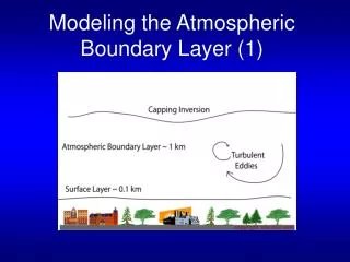
Ice/Ocean Interaction Part 3: The Outer Boundary Layer
Ice/Ocean Interaction Part 3: The Outer Boundary Layer. Ekman ’ s seminal paper Ekman spirals in nature Ekman solution for turbulent stress Neutral IOBL scales, Rossby similarity Scales with stable stratification Scales with destabilizing buoyancy flux. Centripetal acceleration.

Ice/Ocean Interaction Part 3: The Outer Boundary Layer
E N D
Presentation Transcript
Ice/Ocean InteractionPart 3: The Outer Boundary Layer • Ekman’s seminal paper • Ekman spirals in nature • Ekman solution for turbulent stress • Neutral IOBL scales, Rossby similarity • Scales with stable stratification • Scales with destabilizing buoyancy flux
Centripetal acceleration Coriolis acceleration Coriolis Force:
If we are considering a geophysical flow, then for many problems we can ignore the vertical velocity terms, and the Coriolis acceleration becomes simply: Inviscid equation of motion in a rotating reference frame:
h Geostrophy The steady Euler equation in the absence of friction in a rotating reference frame is: For the ocean geostrophic velocity is defined as the horizontal gradient of sea-surface elevation , h, above some reference level.
The Boundary Layer Equation Often the ice and upper ocean layer of turbulently mixed layer are advected by a slowly varying ocean current (the geostrophic current due to sea surface tilt). A good approximation is to express the horizontal momentum equation in terms of the velocity relative to this velocity.
In a steady, horizontally homogeneous flow the volume transport in the frictional boundary layer (relative to the geostrophic flow) is the integral of ur from the bottom of the boundary layer to the top, where the bottom is defined as the level where turbulent stress vanishes. stress Volume transport (northern hemisphere)
Surface air pressure over the Arctic Ocean. Air tends to “fall” away from the center of the high pressure dome, but the earth keeps moving the target, hence the wind deflects to the right. This is evident in the motion of buoys drifting with the sea ice (arrows). High
Inertial Oscillations The time-dependent horizontally homogeneous volume transport equation is: Class Exercise Consider a still ocean subject to a step function wind stress in the y (imaginary) direction. The solution of a nonhomogeneous, linear differential equation is the sum of the homogeneous eqn . solution and a particular solution of the nonhomogeneous eqn.
What is the solution of the steady problem (particular solution)? What is the general solution of the homogeneous 1st order equation? What is the general solution of the nonhomogeneous equation? What is the boundary condition? Sketch the solution.
“On studying the observations of wind and ice-drift taken during the drift of the FRAM, Fridtjof Nansen found that the drift produced by a given wind did not, according to the general opinion, follow the wind’s direction but deviated 20o-- 40o to the right. He explained this deviation as an obvious consequence of the earth’s rotation; and he concluded further that the water-layer immediately below the surface must have a somewhat greater deviation than the latter and so on, since every water-layer is put in motion by the layer immediately above, sweeping over it like a wind…” Ekman Dynamics Ekman, V.W., 1905: On the influence of the earths rotation on ocean currents, Ark. Mat. Astr. Fys., 2, 1-52.
Constitutive law relating stress in the fluid to shear (Ekman postulated that eddy viscosity was independent of depth): 2nd order ordinary differential equation: Boundary conditions: stress at surface specified, velocity vanishes at depth: Steady, horizontally homogeneous boundary layer equation:
B is zero, because V vanishes as General solution: Solve for A:
Ekman’s solution for the steady, unstratified boundary layer forced by stress at the surface of a deep ocean. The net volume transport is perpendicular to the surface stress
In the same paper, Ekman (with credit to Fredholm) also pointed out that the time dependent solutions to the impulsively forced boundary layer equations, included circular oscillations about the mean value, which diminished relatively slowly with depth. Ekman reportedly searched for inertial oscillations in the ocean for all of his long career.
It is mostly overlooked that Ekman came very close to outlining what half a century later became known as Rossby similarity. He related the effective viscosity in the boundary layer to the depth of frictional influence By considering his slope-current arguments and observations of setup and wind speed during storms along the Norwegian continental shelf, he arrived at an expression for D that depended on wind and latitude Had he instead expressed this as In a footnote, he suggested that the eddy viscosity at midlatitudes for a 7 m/s wind would be about 200 cgs (0.02 m2s-1) . Using reasonable estimates of the wind drag coefficient, this means that K* is around 0.02, where Km=K*u*02/f
Hunkins (Deep-Sea Research, 1966) published the first observed example of an Ekman spiral in the ocean, from a composite of current profiles measured from Ice Station Alpha in the Arctic.
Ice Station Weddell, 1992 (McPhee and Martinson, Science, 1994)
Day 365.25 Cluster u* U/u* 1 0.0048 17.9 2 0.0059 16.6
The main criticism of Ekman’s theory is that it did not take into account a thin layer near the surface where shear was much larger than the Ekman solution imposed. In fact, observations show that the turning angle in the boundary layer is typically only about half of the 45o predicted by the constant eddy viscosity. We also saw that in the lower part of the atmospheric boundary layer (the surface layer), λ is linearly dependent on |z|, so K is obviously not constant there. But the atmospheric observers also find that variation of Reynolds stress in the surface layer is small, in fact, they usually ignore its variation with z. So rather than concentrate on velocity in the Ekman layer, suppose we take a similarity approach to turbulent stress instead.
Steady, horizontally homogeneous OBL equation: Define nondimensional variables for stress and vertical coordinate, with the obvious choice for stress the boundary value: Nondimensional momentum equation: Provided
First-order closure (meaning we can express the stress in terms of the velocity derivative in the vertical) Where the nondimensional eddy viscosity is:
Borrowing from Ekman, but with the condition that we are considering turbulent stress, not mean velocity, we assert that K is constant with depth, in which case we can take the derivative of the nondimensional momentum equation to get a 2nd order differential equation. with boundary conditions in the ocean (z positive upward): and the solution is simply where the exponential is complex: the sign indicating the hemisphere, positive north
Nondimensional stress profile from the simple exponential form If the only governing parameters for stress are boundary stress, depth, and the Coriolis parameter (i.e. neglecting buoyancy), the dimensional analysis then dictates that the length scale is the planetary scale: H = u*0/f Then
Similarity and turbulencescales for the neutrally stable outer boundary layer McPhee and Martinson, Science, 1994
During the ISW storm, w and T spectra provided estimates of TKE dissipation rate and temperature variance dissipation rate: ke is a particular wavenumber in the –2/3 region of the kSww(k) spectrum
From the spectra and direct flux measurements, we can make three independent estimates of local mixing length: Where the thermal mixing length comes from equation thermal variance production with thermal dissipation
So we have several ways of getting at the turbulent length scales and eddy viscosity, both at discrete levels: And by three different bulk methods, where the “bulk” in considered constant through the whole layer measured (1) Similarity:
(2) Ekman solution fit where a is the slope of a log-linear fit
By adjusting all of the thermometers on the mast to agree when the mean heat flux is near zero, tiny gradients can be measured. The combination of mast averaged heat flux and temperature gradients provides the bulk thermal eddy diffusivity: Kh = 0.018 m2s-1. (3) Bulk thermal diffusivity
For near neutral stability, the mixing length near the ice/water interface is limited by both the distance from the interface (geometric scale) and by rotation (planetary scale). The former is k|z|, while in my similarity approach the latter limit is L*u*./|f|, where f is the Coriolis parameter. So, in this idealized view, for an instrument clusterat |z|= 2 m where z is measured from the interface, l should look like:
From turbulence mast data obtained during ISPOL in Dec 2004, the mixing length was calculated from the spectral peaks for each 3-hr average, and plotted as a scatter diagram versus the local friction velocity. If the geometric surface layer scale, k|z|, controlled the scale, then for example, at 2 m and 4 m from the interface, the mixing length would follow the yellow and blue horizontal lines respectively. If instead, dynamic boundary layer scaling dominated, the relationship would be indicated by the dashed red line. The heavy dot-dash line is a least-squares regression (through the origin) of l versus u* with light dashed lines indicating confidence limits. The slope is thus indistinguishable from L*/f.
Surface Layer Ekman Layer Rossby similarity, neutrally stable OBL Consider the OBL to comprise mostly an Ekman layer, overlain by a logarithmic “surface” layer through which the stress remains close to the surface value.
Suppose that for the neutral boundary layer the mixing length increases linearly with depth until it reaches a limiting value proportional to u*0/f, and is constant at that value for greater depths: depth l
T0 U0
We end up with a Rossby-similarity drag law for sea ice Where Ro* is the ratio of the planetary scale to the hydraulic roughness of the surface, and the constants A and B are related to the “universal” dimensionless maximum mixing length L*. The sign of iB is negative in the NH, positive in SH.
Drag and turning angle for z0 = 0.03 m, A = 2.3 and B = 2.1 It is standard in most ice models to treat the drag as quadratic: Where is constant, with a constant turning angle between stress and Vs. Using a Rossby-similarity approach, neither is constant
Turbulence scales with stabilizing surface buoyancy flux– MIZEX 1984
Extend the similarity theory developed for the neutrally buoyant Ekman layer to an entire class of Ekman layers including positive (stabilizing) buoyancy flux A simple expression with these asymptotes is half the harmonic mean of the limits: m* is a stability parameter representing the ratio of the planetary scale to the Obukhov length
Now we can form a more general expression for the master length scale H from the stipulation that all the neutral and stably stratified Ekman layers are similar
We have the same dimensionless shear equation with the same complex exponential solution: But now the vertical scale depends not only on u*0/f but also on m*
The velocity profile is integrated in the same was as for the neutral case: