Accelerator Physics Transverse motion

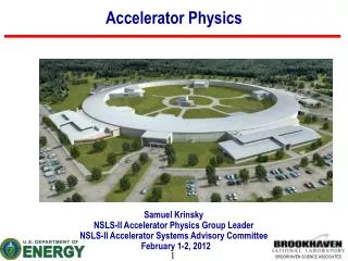
1. Accelerator PhysicsTransverse motion Elena Wildner NUFACT09 School

2. Accelerator co-ordinates Vertical Horizontal Longitudinal It travels on the central orbit 2 Rotating Cartesian Co-ordinate System NUFACT09 School

3. Two particles in a dipole field Particle A Particle B • What happens with two particles that travel in a dipole field with different initial angles, but with equal initial position and equal momentum ? • Assume that Bρis the same for both particles. • Lets unfold these circles…… 3 NUFACT09 School

4. The 2 trajectories unfolded Particle B Particle A displacement 2p 0 • The horizontal displacement of particle B with respect to particle A. • Particle B oscillates around particle A. • This type of oscillation forms the basis of all transverse motion in an accelerator. • It is called ‘Betatron Oscillation’ NUFACT09 School

5. Dipole magnet • A dipole with a uniform dipolar field deviates a particle by an angle θ. • The deviation angle θ depends on the length L and the magnetic field B. • The angle θ can be calculated: • If q is small: • So we can write: NUFACT09 School

6. ‘Stable’ or ‘unstable’ motion ? • Since the horizontal trajectories close we can say that the horizontal motion in our simplified accelerator with only a horizontal dipole field is ‘stable’ • What can we say about the vertical motion in the same simplified accelerator ? Is it ‘stable’ or ‘unstable’ and why ? • What can we do to make this motion stable ? • We need some element that ‘focuses’ the particles back to the reference trajectory. • This extra focusing can be done using: Quadrupole magnets NUFACT09 School

7. Quadrupole Magnet • A Quadrupole has 4 poles, 2 north and 2 south Magnetic field • They are symmetrically arranged around the centre of the magnet • There is no magnetic field along the central axis. Hyperbolic contour x · y = constant NUFACT09 School

8. Resistive Quadrupole magnet NUFACT09 School

9. Quadrupole fields • On the x-axis (horizontal) the field is vertical and given by: By x • On the y-axis (vertical) the field is horizontal and given by: Bx y • The field gradient, K is defined as: • The ‘normalised gradient’,k is defined as: Magnetic field NUFACT09 School

10. Types of quadrupoles • This is a: Focusing Quadrupole (QF) Force on particles • It focusesthe beam horizontallyand defocuses the beam vertically. • Rotating this magnet by 90º will give a: Defocusing Quadrupole (QD) NUFACT09 School

11. Focusing and Stable motion • Using a combination of focusing (QF) and defocusing (QD) quadrupoles solves our problem of ‘unstable’ vertical motion. • It will keep the beams focused in both planes when the position in the accelerator, type and strength of the quadrupoles are well chosen. • By now our accelerator is composed of: • Dipoles, constrain the beam to some closed path (orbit). • Focusing and Defocusing Quadrupoles, provide horizontal and vertical focusing in order to constrain the beam in transverse directions. • A combination of focusing and defocusing sections that is very often used is the so called: FODO lattice. • This is a configuration of magnets where focusing and defocusing magnets alternate and are separated by non-focusing drift spaces. NUFACT09 School

12. FODO cell QF QF QD L2 L1 ‘FODO’ cell Or like this…… Centre of second QF Centre of first QF • The ’FODO’ cell is defined as follows: NUFACT09 School

13. The mechanical equivalent • The gutter below illustrates how the particles in our accelerator behave due to the quadrupolar fields. • Whenever a particle beam diverges away from the central orbit the quadrupoles focus them back towards the central orbit. • How can we represent the focusing gradient of a quadrupole in this mechanical equivalent ? NUFACT09 School

14. The particle characterized x’ x s x ds dx • A particle during its transverse motion in our accelerator is characterized by: • Positionor displacement from the central orbit. • Angle with respect to the central orbit. x = displacement x’ = angle = dx/ds • This is a motion with a constant restoring coefficient, similar to the pendulum NUFACT09 School

15. Hill’s equation These transverse oscillations are called Betatron Oscillations, and they exist in both horizontal and vertical planes. The number of such oscillations/turn is Qx or Qy. (Betatron Tune) (Hill’s Equation) describes this motion If the restoring coefficient (K) is constant in “s” then this is just SHM Remember “s” is just longitudinal displacement around the ring NUFACT09 School

16. Hill’s equation (2) • In a real accelerator K varies strongly with ‘s’. • Therefore we need to solve Hill’s equation for K varying as a function of ‘s’ • The phase advance and the amplitude modulation of the oscillation are determined by the variation of K around (along) the machine. • The overall oscillation amplitude will depend on the initialconditions. NUFACT09 School

17. Solution of Hill’s equation (1) • 2nd order differential equation. • Guess a solution: • εand 0 are constants, which depend on the initial conditions. • (s) = the amplitude modulation due to the changing focusing strength. • (s) = the phase advance, which also depends on focusing strength. NUFACT09 School

18. Solution of Hill’s equation (2) • Define some parameters • …and let Remember  is still a function of s • In order to solve Hill’s equation we differentiate our guess, which results in: • ……and differentiating a second time gives: • Now we need to substitute these results in the original equation. NUFACT09 School

19. Solution of Hill’s equation (3) • So we need to substitute and its second derivative into our initial differential equation • This gives: Sine and Cosine are orthogonal and will never be 0 at the same time NUFACT09 School

20. Solution of Hill’s equation (4) • Using the ‘Sin’ terms , which after differentiating gives • We defined and gives: • Combining Which is the case as: since • So our guess seems to be correct NUFACT09 School

21. Solution of Hill’s equation (5) w b a d ' = = - w b ds 2 • Since our solution was correct we have the following for x: • For x’ we have now: • Thus the expression for x’ finally becomes: NUFACT09 School

22. Phase Space Ellipse x’ x • So now we have an expression for x and x’ and • If we plot x’ versus x we get an ellipse, which is called the phase space ellipse.  = 3/2  = 0 = 2 NUFACT09 School

23. Phase Space Ellipse (2) x’ x’ x x • As we move around the machine the shape of the ellipse will change as  changes under the influence of the quadrupoles • However the area of the ellipse () does not change Area =· r1· r2 •  is called the transverse emittance and is determined by the initial beam conditions. • The units are meter·radians, but in practice we use more often mm·mrad. NUFACT09 School

24. Phase Space Ellipse (3) x’ x’ x x • The projection of the ellipse on the x-axis gives the Physical transverse beam size. • The variation of (s) around the machine will tell us how the transverse beam size will vary. NUFACT09 School

25. Emittance & Acceptance x’ emittance beam x acceptance • Many particles • Observe all the particles at a single position on one turn and measure both their position and angle. • This will give a large number of points in our phase space plot, each point representing a particle with its co-ordinates x, x’. • The emittance is the areaof the ellipse, which contains a defined percentage, of the particles. • The acceptance is the maximum areaof the ellipse, which the emittance can attain without losing particles. NUFACT09 School

26. Matrix Formalism • Lets represent the particles transverse position and angle by a column matrix. • As the particle moves around the machine the values for x and x’ will vary under influence of the dipoles, quadrupoles and drift spaces. • These modifications due to the different types of magnets can be expressed by a Transport Matrix M • If we know x1 and x1’ at some point s1 then we can calculate its position and angle after the next magnet at position S2 using: NUFACT09 School

27. How to apply the formalism • If we want to know how a particle behaves in our machine as it moves around using the matrix formalism, we need to: • Split our machine into separate element as dipoles, focusing and defocusing quadrupoles, and drift spaces. • Find the matrices for all of these components • Multiply them all together • Calculate what happens to an individual particle as it makes one or more turns around the machine NUFACT09 School

28. Matrix for a drift space x2 = x1 + L.x1’ x1’ x1 x1’ small L } • A drift space contains no magnetic field. • A drift space has length L. NUFACT09 School

29. Matrix for a quadrupole deflection x1 x2 x1’ Remember By x and the deflection due to the magnetic field is: x2’ } Provided L is small • Aquadrupoleof length L. NUFACT09 School

30. Matrix for a quadrupole (2) • We found : • Define the focal length of the quadrupole as f= NUFACT09 School

31. A quick recap……. • We solved Hill’s equation, which led us to the definition of transverse emittance and allowed us to describe particle motion in phase space in terms of β,α, etc… • We constructed the Transport Matrices corresponding to drift spaces and quadrupoles. • Now we must combine these matrices with the solution of Hill’s equation to evaluate β,α, etc… NUFACT09 School

32. Matrices & Hill’s equation • We can multiply the matrices of our drift spaces and quadrupoles together to form a transport matrix that describes a larger section of our accelerator. • These matrices will move our particle from one point (x(s1),x’(s1)) on our phase space plot to another (x(s2),x’(s2)), as shown in the matrix equation below. • The elements of this matrix are fixed by the elements through which the particles pass from point s1 to point s2. • However, we can also express (x,x’) as solutions of Hill’s equation. and NUFACT09 School

33. Matrices & Hill’s equation (2) • Assume that our transport matrix describes a complete turnaround the machine. • Therefore : (s2) = (s1) • Let mbe the change in betatron phase over one complete turn. • Then we get for x(s2): NUFACT09 School

34. Matrices & Hill’s equation (3) • So, for the position x at s2 we have… • Equating the ‘sin’ terms gives: • Which leads to: • Equating the ‘cos’ terms gives: • Which leads to: • We can repeat this for c and d. NUFACT09 School

35. Matrices & Twiss parameters Number of betatron oscillations per turn • Remember previously we defined: • These are called TWISS parameters • Remember also that mis the total betatron phase advance over one complete turn is. • Our transport matrix becomes now: NUFACT09 School

36. Lattice parameters • This matrix describes one complete turn around our machine and will vary depending on the starting point (s). • If we start at any point and multiply all of the matrices representing each element all around the machine we can calculate α, β, γ and μfor that specific point, which then will give us β(s) and Q • If we repeat this many times for many different initial positions (s) we can calculate our Lattice Parameters for all points around the machine. NUFACT09 School

37. Lattice calculations and codes • Obviously m (or Q) is not dependent on the initial position ‘s’, but we can calculate the change in betatron phase, dm, from one element to the next. • Computer codes like “MAD” or “Transport” vary lengths, positions and strengths of the individual elements to obtain the desired beam dimensions or envelope ‘β(s)’ and the desired ‘Q’. • Often a machine is made of many individual and identical sections (FODO cells). In that case we only calculate a single cell and not the whole machine, as the the functions β(s) and dμwill repeat themselves for each identical section. • The insertion section have to be calculated separately. NUFACT09 School

38. The b(s) and Q relation. , where μ =Δ over a complete turn • We use: Over one complete turn • This leads to: • Increasing the focusing strength decreases the size of the beam envelope (β)and increases Q and vice versa. NUFACT09 School

39. Tune corrections • What happens if we change the focusing strength slightly? • The Twiss matrix for our ‘FODO’ cell is given by: • Add a small QF quadrupole, with strength dK and length ds. • This will modify the ‘FODO’ lattice, and add a horizontal focusing term: • The new Twiss matrix representing the modified lattice is: NUFACT09 School

40. Tune corrections (2) • This gives • This extra quadrupole will modify the phase advance  for the FODO cell. 1 =  + d New phase advance Change in phase advance • If d is small then we can ignore changes in β • So the new Twiss matrix is just: NUFACT09 School

41. Tune corrections (3) • Adding and compare the first and the fourth terms of these two matrices gives: • These two matrices represent the same FODO cell therefore equals: NUFACT09 School

42. Tune corrections (4) QD QF Remember 1 =  + d and dμ is small dQ = dμ/2π ,but: In the horizontal plane this is a QF If we follow the same reasoning for both transverse planes for both QF and QD quadrupoles NUFACT09 School

43. Tune corrections (5) Let dkF = dk for QF and dkD = dk for QD bhF, bvF = b at QF and bhD, bvD = b at QD Then: This matrix relates the change in the tune to the change in strength of the quadrupoles. We can invert this matrix to calculate change in quadrupole field needed for a given change in tune NUFACT09 School

44. Acknowledgements Acknowldements to • Simon Baird, • Rende Steerenberg, • Mats Lindroos, for course material NUFACT09 School