AS - AD
AS - AD. AS - AD. Aggregate Supply relates output and price level labor market Aggregate Demand relates output and price level IS - LM. Aggregate Supply. As output rises…. P = W(1 + m ) W = P e F ( u,z ) P = P e (1 + m )F( u,z ) For fixed P e , as Y rises, u falls so P rises


AS - AD
E N D
Presentation Transcript
AS - AD • Aggregate Supply • relates output and price level • labor market • Aggregate Demand • relates output and price level • IS - LM
Aggregate Supply As output rises…. P = W(1 + m) W = PeF(u,z) P = Pe(1 + m)F(u,z) For fixed Pe, as Y rises, u falls so P rises why? Hiring pushes up wages. Note: Pe fixed in the short run.
AS (in detail) U – number of workers unemployed N – workforce (constant) L - workers employed U = N - L Unemployment rate u = (N - L)/N =1-L/N Production function Y=AL A – productivity u = 1-Y/(AN)
AS (in detail) P = Pe(1 + m)F(u,z) u = 1-Y/(AN) P = Pe(1 + m)F(1-Y/(AN),z) AS relation, as Y↑ u↓ u↓ F(u,z)↑ F(u,z) ↑ P↑ So AS is upward sloping
AS • Slopes up • Shifts • Change in Pe • Rise in expectations • Shifts AS up • Productivity A↑ AS shifts right/down • Markup m↑ AS shifts up • Change in z, labor market conditions
Aggregate Demand • How does a price increase affect equilibrium GDP on an IS – LM graph. • LM shifts up (left) • Y* falls • AD slopes down • Shifts – anything else that affects IS – LM • Autonomous spending • Policy (both kinds) • Exception – supply side tax effects
Problems • Show how an increase in the money supply would affect the equilibrium level of output, interest rates and prices using and IS – LM and AS – AD diagram. • The 1990s saw an increase use of IT in business which improved productivity. Show the short run effect on an AS-AD graph.
Problems Show how an decrease in government spending would affect the equilibrium level of output, interest rates and prices using and IS – LM and AS – AD diagram. Show the effect of an increase in oil prices has on an AS-AD graph.
Medium Run • Expectations adjust • P=Pe • Unemployment at its natural rate 1 = (1 + m)F(un,z) • Output at its natural rate un= 1-Yn/(AL) AS? 1 = (1 + m)F(1-Yn/(AL),z) Vertical at the natural rate of output
Medium run • What if Y* < Yn ? • P < Pe (short run) • medium run, Pefalls to P • AS shifts down/right • Y* rises to Yn • Labor Market interpretation • u* > un • as Pefalls, wages bid down • lower cost to production • AS shifts right • Medium run Y* =Yn
Monetary policy: short and medium run • Fed increase Ms • AD shifts right • Y* and P* both rise • short run (P > Pe) • Medium run • Pe rises • AS shifts up/left • Y* falls back to Yn • P* rises further • Money neutrality (med run) • changes in Ms • affect nominal variables • not real variables
Problem Show how a decrease in the money supply would affect the equilibrium output and price levels on an AS-AD graph in the short and medium run. What happens on the IS-LM graph in the short and medium run?
Problems AS-AD Show the short and medium run effects of an increase in productivity. Show the short and medium effects of a decrease in consumer confidence. Show the short and medium run effects of an increase in oil prices.
Recessionary Gap Y* < Yn Inflationary Gap Y*> Yn Show an inflationary gap on an AS-AD graph, then show how the government could use tax policy to close the gap. Show a recessionary gap on an AS-AD graphs, then show how monetary policy could be used to close the gap.
Gov’t Spending How does an increase in government spending affect the AS-AD graph in the short & medium run? Does Gov’t spending affect productivity? Show the changes in the graph for both cases.
Key Equations P = W(1 + m) (PS) W = PeF(u,z) (WS) 1 = (1 + m)F(un,z) u = 1-Y/(AL) P = Pe(1 + m)F(1-Y/(AL),z) (AS)
Unemployment & Inflation Inverse relation Can the Fed lower U? Increase MS If inflation is caused by AD shift to the right output rises, unemployment falls Fed can lower U at a cost of higher p True? Check the data.
Inflation versus Unemploymentin the United States, 1948-1969
Inflation versus Unemploymentin the United States since 1970
PC relation to WS W = PeF(u,z) (WS) P = W(1 + m) (PS) Let F(u,z) = 1 – au + z So WS & PS become P = Pe(1 + m)(1 – au + z) Do some math…. • = pe + m - au + z inverse relation does exist
Wage – Price Spiral Explains inverse relation • u falls • wages bid up • prices rise • workers demand higher wages • etc. etc. • higher p “Tight labor market” – late 1990s
Shifts in PC • Expectations • markup • input costs • market power • labor market condtions • Anything that shifts AS, shifts PC
Medium Run PC equation in the medium run? expectations equal inflation un depends only on m, z, a
Monetary Policy and the PC The Fed tries to lower u below the natural rate….. Show on AS-AD and the PC for the short and medium run.
Review Problems Show a Phillips curve graph and an AS-AD graph starting from an inflationary gap. Show the medium run adjustment. If the Fed acts to close an inflationary gap, what would they do? Show the result on an AS-AD graph and a PC graph.
Story of the Great Inflation • Productivity falls • oil prices rise • Effect on Yn, un • Monetary policy reaction • Fed tried to keep u at the old level • expectations rose Both shifts and a return to the natural rate
Mr. Burn’s brain What’s behind the Fed’s decisions in the 70’s? • Bad thinking • Ignoring natural rates • Expectations • “old” PC • Bad data • Couldn’t see the change in the natural rates • Cared more about unemployment than inflation
Intellectual history & the PC • “Old” PC (1940-50s) • Empirical relationship • Use in Cowles commission models • Edmund Phelps / Milton Friedman (late 60s) • Argue against the permanent output/inflation tradeoff • 70s proved them right • “Old Keynesian” econometric models abandoned
Expectations and the PC pt = pte + m - aut + z Static expectations pte = pt-1 Rational expectations pte = pt + et et – forecast error
Policy Effectiveness Under rational expectations, what happens when the Fed increases the money supply? PC and AS vertical (with an error term) P & p rise, not real effect Money is neutral. Policy is ineffective. Why?
Problem Starting from the natural rate of unemployment, if the Fed acts to lower inflation, show the SR & MR effects.
Equations P=Pe(1+m)F(u,z) W = PeF(u,z) p = pe + m - au + z P = W(1+m) M/P = L(i,Y) un = (m + z)/a
Equations P=Pe(1+m)F(u,z) AS (sort of) W = PeF(u,z) WS p = pe + m - au + z SRPC P = W(1+m) PS M/P = L(i,Y) Money Demand un = (m + z)/a MRPC/natural rate of u
More Review The government becomes more aggressive about breaking up monopolies lowering the pricing power of firms. Show the impact on the following graphs. • real wage / unemployment • AS – AD • Phillips curve • IS – LM
More Review The recent housing market decline led to an decrease in autonomous consumption and investment. Show that short run change and the medium run adjustment, assuming passive policy on the following graphs: • IS-LM • AS-AD • Phillips Curve
Review problem Show an inflationary gap on graphs of AS-AD and IS-LM. Use the graph to explain how tax policy could be used to close the gap..
Review Problem Show the short run effect of a tax increase on an expenditure diagram. Show the short and medium effects on IS-LM and AS-AD diagrams.
Review Problem Keynes once advocated that the government should bury boxes of money and let people dig them up to stimulate to economy. Starting from the natural rates or unemployment and output, show the short and medium run effects of an increase in government spending that does not change the natural rates for AS-AD and the Phillip’s curve.
Review Problem Currently the Fed is increasing the money supply and keeping interest rates low to mitigate the recession. Starting from a recessionary gap, show the effect of an increase in the money supply on an AS-AD graph and the Phillip’s Curve.
Practice Problem The financial crisis has led to a decrease in lending and therefore an fall in the money supply. Starting from the natural rates of output and unemployment, show the resulting change on AS-AD and Phillips curve graphs in the short run.
Goals • Connect output, unemployment and inflation • Use equations • Explain both short and medium runs y, u and p Actually, we’ll use gy – growth rate
Okun’s Law Connects u and y ut – ut-1 = - b(gy,t – gn) gn - “normal” or natural growth rate of output - growth rate of potential GDP
Phillips Curve Connects p and u • = pe + m - au + z or pt - pet = a(un - ut) Related to AS
p and Y Focus on AD and monetary policy M/P rises, LM & AD shift right Y rises Let Y = g(M/P) Assumes fiscal policy and autonomous expenditures are fixed. Log differencing the equation: gy,t = gm,t - pt
small macro model ut – ut-1 = - b(gy,t – gn) pt - pet = a(un - ut) gy,t = gm,t – pt MR implications: • = pe ; u = un ; gy,t = gn pt = gm,t – gn