Mastering MATLAB Matrices: Manipulation, Extraction, & Problem Solving
550 likes | 606 Vues
Learn to manipulate matrices, extract data, solve problems with two variables, & explore special matrices in MATLAB. Practice defining matrices, indexing, and using the colon operator for efficient matrix operations.

Mastering MATLAB Matrices: Manipulation, Extraction, & Problem Solving
E N D
Presentation Transcript
Objectives After studying this chapter you should be able to: • Manipulate matrices • Extract data from matrices • Solve problems with two variables • Explore some of the special matrices built into MATLAB
Section 4.1Manipulating Matrices • We’ll start with a brief review • To define a matrix, type in a list of numbers enclosed in square brackets
Remember that we can define a matrix using the following syntax • A=[3.5] • B=[1.5, 3.1] or • B=[1.5 3.1] • C=[-1, 0, 0; 1, 1, 0; 0, 0, 2];
2-D Matrices can also be entered by listing each row on a separate line C = [-1, 0, 0 1, 1, 0 1, -1, 0 0, 0, 2]
Use an ellipsis to continue a definition onto a new line F = [1, 52, 64, 197, 42, -42, … 55, 82, 22, 109];
These semicolons are optional 2-D matrix
If you add an element outside the range of the original array, intermediate elements are added with a value of zero
4.1.2 Colon Operator • Used to define new matrices • Modify existing matrices • Extract data from existing matrices
Evenly spaced vector The default spacing is 1
User specified spacing The spacing is specified as 0.5
All the rows in column 1 All the rows in column 4 All the columns in row 1 The colon can be used to represent an entire row or column
Rows 2 to 3, all the columns You don’t need to extract an entire row or column
A single colon transforms the matrix into a column MATLAB is column dominant
Indexing techniques • To identify an element in a 2-D matrix use the row and column number • For example element M(2,3)
Or use single value indexing M(8) is the same element as M(2,3) Element #s
The word “end” signifies the last element in the row or column Row 1, last element Last row, last element Last element in the single index designation scheme
Section 4.2Problems with Two Variables • All of our calculations thus far have only included one variable • Most physical phenomena can vary with many different factors • We need a strategy for determining the array of answers that results with a range of values for multiple variables
When you multiply two vectors together, they must have the same number of elements
Array multiplication gives a result the same size as the input arrays x and y must be the same size
Distance to the horizon Distance to the horizon, d Height of the mountain Radius plus the height of the mountain, R+h Radius of the earth, R Radius of the earth Example 4.2Distance to the Horizon
State the problem • Find the distance to the horizon from the top of a mountain on the moon and on the earth
Describe the Input and Output • Input • Radius of the Moon 1737 km • Radius of the Earth 6378 km • Mountain elevation 0 to 8000km • Output • Distance to the horizon in km
Hand Example Pythagorean theorum Solve for d Using the radius of the earth, and an 8000 meter mountain. (Remember 8000m = 8 km)
Test the Solution • Compare the results to the hand solution
Section 4.3Special Matrices • zeros • Creates a matrix of all zeros • ones • Creates a matrix of all ones • diag • Extracts a diagonal or creates an identity matrix • magic • Creates a “magic” matrix
With a single input a square matrix is created with the zeros or ones function
When the input argument to the diag function is a square matrix, the diagonal is returned The diag function
When the input is a vector, it is used as the diagonal of an identity matrix The diag function
This woodcut called Melancholia was created by Albrect Durer, in 1514. It contains a magic matrix above the angel’s head
Durer switched these two columns to make the date work out The Durer matrix is different from MATLAB’s 4x4 magic matrix
Summary • Matrices can be created by combining other matrices • Portions of existing matrices can be extracted to form smaller matrices