Constrained Scheduling in Directed Acyclic Graphs with Precedence Constraints
This document presents a comprehensive study on constrained scheduling within directed acyclic graphs (DAGs) while considering precedence constraints. It outlines the problem of minimizing schedule length using p processors (workmen) and describes algorithms, their complexities, and results. Key findings highlight the poly-time algorithm for two processors and the NP-hard nature of variable processor numbers. Additionally, the paper discusses techniques for deadline management and presents approximation algorithms, emphasizing their applications in project management and parallel computing.


Constrained Scheduling in Directed Acyclic Graphs with Precedence Constraints
E N D
Presentation Transcript
Precedence Constrained Scheduling Abhiram Ranade Dept. of CSE IIT Bombay
Input • Directed Acyclic Graph G, #processors p A G E , 3 B F H C Vertex = unit time task edge (u,v) : Time(u) < Time(v) D
Output: Schedule Time 1 2 3 4 Processor 1 A D E G Processor 2 B F H Processor 3 C Schedule Length, to be minimized
Applications Project management. Vertex = lay foundation, build walls. Edges: what happens first to what happens later. Processors : Number of workmen. MS Project, others. Our problem: Simplified version. Other applications: Parallel computing.
Summary of results • Polytime algorithm when p=2. [Fuiji.. 69] • NP-hard for variable p. [LenKan 78] • NP-hardness not known for fixed p > 2. • Polytime algorithm for trees. [Hu 61]
Summary of results - 2 • Any greedy algorithm gives 2 - 1/p approximation. i.e. Schedule of length at most (2 - 1/p) times Optimal length. • [Coffman-Graham 72, Lam-Sethi 77] give 2 - 2/p approximation algorithm. • [Gangal-Ranade 08] give 2 – 7/(3p+1) approximation for p > 3. • [Svensson 10] Better than 2-ε unlikely.
Outline • Elementary Lower Bound ideas • Elementary algorithm and analysis • Deadline Constraints [GarJoh 76] • More complex problem, but generates new ideas. • 2 processor optimality, also without deadlines • Essentially gives 2 - 2/p approximation • Ideas behind 2 - 7/(3p+1) approximation algorithm
Elementary Lower Bounds • To prove optimality of any algorithm, need to show why it cannot be improved, i.e. lower bound on schedule length. • OPT H = Length of longest path in G. • OPT [ N / p ], N = #nodes [ x ] = ceiling(x), smallest integer x. Example: H = 3, [N/p] =[8/3] = 3
Input • Directed Acyclic Graph G, #processors p A G E , 3 B F H C Vertex = unit time task edge (u,v) : Time(u) < Time(v) D
Generic Algorithm • Pick any “ready” vertex. • Schedule it at earliest possible time. • Repeat until done. ready = no predecessors yet unscheduled. earliest possible = after predecessors.
Proof of 2 approximation • Full (time) slot: All processors busy • Number of “full” slots N/p • Number of partial slots H. Why? • Partial slot: Some processor did not get work. • All maximally long paths must shrink. • This can happen only H times. • Time N/P + H OPT + OPT = 2 OPT • Improve to 2 - 1/p.
Deadline Constraints [GarJoh 76] • Additional Input: D(v) : time by which v must be processed. • Need a schedule with p processors in which precedence constraints and deadlines are respected.
Deadline Propagation • v has N(d) descendants with deadline d v must itself finish by d - [N(d)/p]. new deadline: d(v) = min( D(v), mind d -[N(d)/p] ) • In what order to calculate? • (u,v) edge d(u) < d(v) • GJ Algo: priority = deadline. Optimal for p=2!
Example 4 4 d(A) = 4 - [7/5] = 2 d(B) = min(4-[8/5], 2-[1/5]) = 1 d(C) = …. = 3 d(D) = = 2 d(E) = . . . = 0 . B A . E D C . . 4
GJ Deadline Properties • Deadline < 1 : schedule not possible. • Optimal Schedule length Max deadline - Min deadline + 1. • Opt for example 4 - 0 + 1 = 5 • Load bound : [N/p] = [17/5] = 4 • Longest path: H = 4 • Is this the best lower bound?
Partial Slot Bound Max Deadline – Min Deadline + 1 >= H Time 1 2 . . . t . . . . . P1 u v P2 - u is ancestor of v, so d(u) < d(v)
Load Bound Max deadline – Min deadline + 1 >= [N/p] Add a universal parent z d(z) <= Max deadline – [Number of descendants with deadline d/p] = Max – [N/p] Min deadline <= Max – [N/p]
Scheduling without deadlines • Set d(terminal vertices) = k, some number. • Propagate deadlines. m = least deadline. • Schedule from time m using deadlines. Theorem: Algorithm is optimal for p=2.
2 Processor Optimality • v : earliest scheduled vertex not meeting deadline • w : latest scheduled vertex before v scheduled alone. Always exists? Nodes in region must be Descendants of w. Time: 1 2 3 t’ t Proc 1: w v Proc 2: - Region has 2(t-t’)-1nodes with Deadline t-1. • d(w) t’, d(v) t-1 d(w) t-1 - (2(t-t’)-1)/2 = t’-1 Contradiction
Remarks • Why does this not work for p > 2? • Algorithm gives 2 - 2/p approximation for even p. More complex proof.
Improvements to GJ [GR 09] • Node v has N(d,L) descendants at distance at least L+1 having deadline at least d • Then d(v) mind,L d - L - [N(d,L)/p]
Example 4 d(A) = 4 - [7/5] = 2 d(B) = min(4-[8/5], 2-[1/5]) = 1 d(C) = …. = 3 d(D) = = 2 d(E) = . . . = 0 d(E) 4 – 2 – [12/5] = -1 Max - min + 1 = 6.Optimal! 4 . B A . E D C . . 4
Algorithm • Set d(terminal vertices) = 0 • Propagate deadlines. New rule. • For each v in non-decreasing deadline order: • (Rearrange ancestors of v if possible). • Schedule v in earliest possible slot, and smallest numbered processor.
Rearrange ancestors of v • Suppose t = last slot with ancestors of v. • Suppose vertices in slots t-1,t have same deadline. • Suppose v has < p ancestors in t-1,t. • Then move ancestors of v to slot t-1, move other vertices to slot t. • If slot t is not full, v can be scheduled in t.
Analysis Outline • Key part of proof: If algorithm constructs a long schedule, then deadline must drop a lot moving from last column to first. • Max deadline - min deadline + 1 optimal schedule length. • Optimal schedule must also be long, so good approximation factor.
How deadline varies in the schedule Time> 1 2 3 …. u v w 1 2 3 . . p Deadline can only increase in first row: D(u) D(v) Deadline can only increase in any column: D(u) D(w)
Partial slot rule 1 2 3 ….increasing time. u v w x y - - 1 2 3 . . p Deadline must increase in first row after a partial slot: D(u) < D(v) … why was not v scheduled earlier?
1-slot rule 1 2 3 ….increasing time. u v - - - - - 1 2 3 . . p Let M denote the number of nodes scheduled after u. Then D(u) D(v) - [M/p]
Intuition: Easy schedules • Suppose all slots are partial: drop per slot. • Thus total deadline drop = length of schedule. • Optimal! • Suppose all slots are either 1 slots or full slots. • 1-slot rule gives optimality.
Intuition: Difficult Schedules • Schedules with mixture of 2-slots and full slots. • Extreme case 1: 2-slots at the beginning, full slots at the end. • Extreme case 2: 2 slots and full slots alternate.
Extreme case 1: • Time> <--L--> <---m--> • P1 : a v v v v v v v v v w • P2 : b v v v v v v v v v • P3 : v v v v v • P4 : v v v v v • A,b must be ancestors of all to right. • One of them say a, must be ancestor of mp/2 • d(a) d(w) - L - mp/2. • Drop = #2slots + full slots/2
Extreme Case 2 • Time:1 2 3 4 5 . . . . • P1 : v v v v v v • P2 : v v v v v v • P3 : v v v • P4 : v v v • Use ancestor rearrangement to argue large drop.
Actual Analysis • Keep track of how many 1-slots, 2-slots, full slots .. encountered. • Relate numbers to deadline drop, schedule length. • Solve for schedule length/deadline drop.
Remarks • Analysis is complicated, but not much more than 2-2/p analysis of Lam-Sethi. • Algorithm is simpler than Coffman-Graham. • Technique will not work beyond 2 - 3/p. Even getting there is hard.


![W[2]-hardness of precedence constrained K-processor scheduling](https://cdn1.slideserve.com/3323938/w-2-hardness-of-precedence-constrained-k-processor-scheduling-dt.jpg)