Download
1 / 51
510 likes | 896 Vues
AFNI Soup to Nuts: How to Analyze Data with AFNI from Start to Finish. There is no single “correct” way to analyze fMRI data. The path your data takes will depend on the quality of the data, the complexity of the experiment, and the needs of the researcher.

E N D
AFNI Soup to Nuts:How to Analyze Data with AFNI from Start to Finish • There is no single “correct” way to analyze fMRI data. The path your data takes will depend on the quality of the data, the complexity of the experiment, and the needs of the researcher. • However, there are some typical processing steps that are widely used. These steps are introduced and discussed in this handout. • All processing steps will be done with AFNI (hence, AFNI “soup to nuts”). • The sample study used for this hands-on is a real study, although the variable names have been slightly modified. • afni_proc.py • The data processing script discussed in this handout was generated by a program in AFNI calledafni_proc.py. • Specifically,afni_proc.pyis a python script that can generate a single-subject data analysis script by asking the user to provide information regarding their study, such as input datasets and stimulus files that will be used. The program also asks for more specific information, such as the number of TRs to be removed (if any), the EPI volume that will be used to align the remaining volumes, and additional information necessary for the regression or deconvolution analysis that will follow.
At the moment, this information is input via a command-line interface, or with an optional question/answer session (afni_proc.py -ask_me). Eventually, a GUI will become available (but not yet). • Onceafni_proc.pyhas all the necessary information, it produces a tcsh (T-shell) script that contains all the data processing steps. This script can be easily executed and the end result will be a functional/statistical dataset, as well as numerous datasets produced from the intermediary steps. • Before we go any further, start the processing script: • we will discuss it more, soon • under AFNI_data4, execute the script containing the afni_proc.py command • this will create the processing script, proc.sb23.blk • execute the proc.sb23.blk script, as recommended by afni_proc.py • takes ~4 minutes on my laptop cd AFNI_data4 tcsh s1.afni_proc.block tcsh -x proc.sb23.blk |& tee output.proc.sb23.blk
The Experiment: • Cognitive Task: Subjects see photographs of two people interacting. • The mode of communication falls in one of 3 categories: via telephone, email, or face-to-face. • The affect portrayed is either negative, positive, or neutral in nature. • Experimental Design: 3x3 Factorial design, BLOCKED trials • Factor A: CATEGORY - (1) Telephone, (2) E-mail, (3) Face-to-Face • Factor B: AFFECT - (1) Negative, (2) Positive, (3) Neutral • A random 30-second block of photographs for a task (ON), followed by a 30-second block of the control condition of scrambled photographs (OFF), and so on. • Each run has 3 ON blocks, 3 OFF blocks. There are 9 runs in a scanning session.
AFFECT Negative Positive Neutral • Illustration of Stimulus Conditions: “You are the best project leader!” “Your project is lame, just like you!” “You finished the project.” Telephone CATEGORY "Your new haircut looks awesome!" "Ugh, your hair is hideous!" "You got a haircut." E-mail “I curse the day I met you!” “I feel lucky to have you in my life.” “I know who you are.” Face-to-Face • Data Collected: • 1 Anatomical (MPRAGE) dataset for each subject • 124 axial slices • voxel dimensions = 0.938 x 0.938 x 1.2 mm • 9 Time Series (EPI) datasets for each subject • 34 axial slices x 67 volumes = 2278 slices per run • TR = 3 sec; voxel dimensions = 3.75 x 3.75 x 3.5 mm • Sample size, n=16 (all right handed)
Analysis Steps: • Part I: Process data for each individual subject (using afni_proc.py) • Pre-process subjects’ data many steps involved here… • Run regression analysis on each subject’s data ---3dDeconvolve • Part II: Run group analysis • warp results to standard space • 3-way Analysis of Variance (ANOVA) ---3dANOVA3 • Category (3) x Affect (3) x Subjects (16) => 3-way ANOVA • Class work for Part I: • view the original data by running afni from the subjectsb23/directory • then view output data from thesb23.blk.results/directory cd AFNI_data4/sb23 ls afni &
Back to afni_proc.py: • For our class example, we can take a look at the afni_proc.py command we’ve written up already and saved as an executable script called s1.afni_proc.block (perhaps viewing in a different terminal window) cd AFNI_data4 gedit s1.afni_proc.block • note: gedit is a text editor (can also use nedit, emacs or vi) afni_proc.py \ -subj_id sb23.blk \ -dsets sb23/epi_r??+orig.HEAD \ -copy_anat sb23/sb23_mpra+orig \ -tcat_remove_first_trs 3 \ -volreg_align_to last \ -regress_make_ideal_sum sum_ideal.1D \ -regress_stim_times sb23/stim_files/blk_times.*.1D \ -regress_stim_labels tneg tpos tneu eneg epos \ eneu fneg fpos fneu \ -regress_basis 'BLOCK(30,1)' \ -regress_opts_3dD \ -gltsym 'SYM: +eneg -fneg' \ -glt_label 1 eneg_vs_fneg \ -gltsym 'SYM: 0.5*fneg 0.5*fpos -1.0*fneu' \ -glt_label 2 face_contrast \ -gltsym ‘SYM: tpos epos fpos -tneg -eneg -fneg’ \ -glt_label 3 pos_vs_neg
Line-by-Line Explanation of s1.afni_proc.block command: • -subj_id:Specify a subject ID name for the processing script that will be created by executing the s1.afni_proc.block script. The ID in this example is sb23.blk • -dsets: Specify the name of the time series datasets that will be analyzed, as well as the directory path in which they reside. Here, they are called epi_r03+orig ..epi_r11+orig, residing in directory sb23/ (note that .HEAD is required for wildcard matching) • -copy_anat: This option will take the anatomical dataset sb23_mpra+orig that currently resides in sb23/ and copy it into the results directory (the results directory will be created once the processing script has been run) • tcat_remove_first_trs: This option removes ‘x’ number of timepoints from the beginning of each time series run. Here, we have chosen to remove the first 3 timepoints from each run • -volreg_align_to: This volume registration option asks the user to choose which volume will be the base by which all other volumes in the time series runs are aligned. Here we have chosen the last volume from the last epi run (run 9) • -regress_make_ideal_sum: Sums the ideal response curves from the regressors and saves as a 1D file, e.g., sum_ideal.1D • -regress_stim_times: Specifies the name and location of the stimulus timing files for our experiment. In this example, they are sb23/stim_files/blk_times.*.1D
Line-by-Line Explanation of s1.afni_proc.block command (cont…) • -regress_stim_labels: Specifies the names of our 9 regressors:tneg, tpos, tneu, eneg, epos, eneu, fneg, fpos, and fneu • -regress_basis: Specifies the regression basis function to be used by3dDeconvolvein the regression step. In this example, we have'BLOCK(30,1)’, which is a 30-second BLOCK response function (with a peak of 1). • -regress_opts_3dD: Allows for additonal3dDeconvolveoptions, such as general linear tests (glt’s) • We have previously executed the afni_proc.py script, s1.afni_proc.block. (already done) tcsh s1.afni_proc.block • The result is an auto-generated processing script calledproc.sb23.blk. Use a text editor like gedit, nedit, emacs, or vi to open and view this new script: gedit proc.sb23.blk • You will notice that scriptproc.sb23.blkincludes multiple processing steps for the data, including volume registration, blurring, data scaling, and much more. Each step is run by an AFNI program. The next section (Part I) will go over each processing step in detail.
PART I Process Data for each Individual Subject: • Hands-on example: Subjectsb23 • Data Processing Script created by afni_proc.py program:proc.sb23.blk • We will begin with sb23’s anatomical dataset and 9 time-series (3D+time) datasets: sb23_mpra+orig, sb23_mpra+tlrc, epi_r03orig, ED_r04+orig … epi_r11+orig • Below issb23_r03+orig(3D+time) dataset. Notice the first few time points of the time series have relatively high intensities*. We will need to remove them later: First 2-3 timepoints have higher intensity values • Images obtained during the first 4-6 seconds of scanning will have much larger intensities than images in the rest of the timeseries, when magnetization (and therefore intensity) has decreased to its steady state value
Pre-processing is done by the proc.sb23.blk script within the directory, AFNI_data4/sb23.blk.results/. • open the proc.sb23.blk script in an editor (such as gedit), and follow the script while viewing the results • also, go to the sb23.blk.results directory to start viewing the results • starting from thesb23/directory (from the previous slides)… cd .. gedit proc.sb23.blk & cd sb23.blk.results ls afni & • note that in the script, the count command is used to set the $runs variable as a list of run indices: • set runs = ( `count -digits 2 1 9` ) becomes (by the shell quietly executing the count command): • set runs = ( 01 02 03 04 05 06 07 08 09 ) • And so: • foreach run ( $runs ) becomes (when the shell expands the $runs variable): • foreach run ( 01 02 03 04 05 06 07 08 09 )
STEP 0 (tcat): Apply 3dTcat to copy datasets into the results directory, while removing the first 3 TRs from each run. • The first 3 TRs from each run occurred before the scanner reached a steady state. 3dTcat -prefix $output_dir/pb00.$subj.r01.tcat \ sb23/sb23_r03+orig'[3..$]' • The output datasets are placed into $output_dir, which is the results directory. • Using sub-brick selector '[3..$]' sub-bricks 0, 1, and 2 will be skipped. • The '$' character denotes the last sub-brick. • The single quotes prevent the shell from interpreting the '[' and '$' characters. • The output dataset name format is: pb00.$subj.r01.tcat (.HEAD / .BRICK) • pb00 : process block 00 • $subj : the subject ID (sb23, in this case) • r01 : EPI data from run 1 • tcat : the name of this processing block (according to afni_proc.py) (other block names are tshift, volreg, blur, mask, scale, regress)
STEP 1 (tshift): Check for possible “outliers” in each of the 9 time series datasets using 3dToutcount . Then perform temporal alignment using 3dTshift. • An outlier is usually seen as an isolated spike in the data, which may be due to a number of factors, such as subject head motion or scanner irregularities. • The outlier is not a true signal that results from presentation of a stimulus event, but rather, an artifact from something else -- it is noise. foreach run (01 02 03 04 05 06 07 08 09) 3dToutcount -automask pb00.$subj.r$run.tcat+orig \ > outcount_r$run.1D end • How does this program work? For each time series, the trend and Median AbsoluteDeviation are calculated. Points far away from the trend are considered outliers. • "far away" is defined as at least 5.219*MAD (for a time series of 64 TRs) • see 3dToutcount -help for specifics • -automask: does the outlier check only on voxels within the brain and ignores background voxels (which are detected by the program because of their smaller intensity values) • > : redirects output to the text file outcount_r01.1D (for example), instead of sending it to the terminal window.
Note: “1D” is used to identify a numerical text file. In this case, each file consists a column of 64 numbers (b/c of 64 time points). • Subject sb23’s outlier files: outcount_r01.1D outcount_r02.1D … outcount_r09.1D • Use AFNI 1dplot to display any one of ED’s outlier files. For example: 1dplot outcount_r08.1D Number of ‘outlier’ voxels, per TR Outliers? Inspect the data. High intensity values in the beginning are usually due to scanner attempting to reach steady state. Time
in afni, view run 01, time points 38, 39 and 40 • while it appears that something happened at time point 39 - such as a swallow, sneeze, or similar movement - it may not be enough to worry about • if there had been a more significant problem, and if it could not be fixed by3dvolreg, then it might be good to censor this time point via the-censoroption in3dDeconvolve internal movement can be seen in this area, using afni Big spike at timepoint 39
Next, perform temporal alignment using 3dTshift. • Slices were acquired in an interleaved manner (slice 0, 2, 4, …, 1, 3, 5, …). • Interpolate each voxel's time series onto a new time grid, as if each entire volume had been acquired at the beginning of the TR (TR=3 seconds in this example) • For example, slice #0 was acquired at times t = 0, 3, 6, 9, etc., in seconds. However, slice #1 was acquired at times t = 1.5, 4.5, 7.5, 10.5, etc., which is asynchronous with the TR. • After applying 3dTshift, all slices will have offset times of t = 0, 3, 6, etc. 3dTshift -tzero 0 -quintic \ -prefix pb01.$subj.r$run.tshift \ pb00.$subj.r$run.tcat+orig • -tzero 0 : the offset for each slice is set to the beginning of the TR • -quintic : interpolate using a 5th degree polynomial
Subject sb23’s newly created time shifted datasets: pb01.sb23.blk.r01.tshift+orig (.HEAD/.BRIK) ... pb01.sb23.blk.r09.tshift+orig (.HEAD/.BRIK) • Below is run 01 of sb23’s time shifted dataset. Slice acquisition now in synchrony with beginning of TR
STEP 2: Register the volumes in each 3D+time dataset using AFNI program 3dvolreg. • All volumes will be registered to the last volume of the last run (i.e., run 9, volume 63). This volume is closest in proximity to the anatomical dataset. foreach run ( $runs ) 3dvolreg -verbose -zpad 1 \ -base pb01.$subj.r09.tshift+orig'[63]' \ -1Dfile dfile.r$run.1D \ -prefix pb02.$subj.r$run.volreg \ pb01.$subj.r$run.tshift+orig end cat dfile.r??.1D > dfile.rall.1D • -verbose : prints out progress report onto screen • -zpad : add one temporary zero slice on either end of volume • -base : align to last volume, since anatomy was scanned after EPI • -1Dfile : save motion parameters for each run (roll, pitch, yaw, dS, dL, dP) into a file containing 6 ASCII formatted columns • -prefix : output dataset names reflect processing step 2 (volreg) • input datasets are from processing step 1 (tshift) • concatenate the motion parameters (dfiles) from all 9 runs into one file
Subject sb23’s 9 newly created volume registered datasets: pb02.sb23.blk.r01.volreg+orig (.HEAD/.BRIK) ... pb02.sb23.blk.r10.volreg+orig (.HEAD/.BRIK) • Below is run 01 of sb23’s volume registered datasets.
view the registration parameters in the text file, dfile.rall.1D • this is the concatenation of the registration files for all 9 runs 1dplot -volreg dfile.rall.1D • Slight movements going on here, especially at the “Pitch” angle
STEP 3: Apply a Gaussian filter to spatially blur the volumes using program 3dmerge. • result is somewhat cleaner, more contiguous activation blobs • also helps account for subject variability when warping to standard space • spatial blurring will be done on sb23’s time shifted, volume registered datasets foreach run ( $runs ) 3dmerge -1blur_fwhm 4.0 -doall \ -prefix pb03.$subj.r$run.blur \ pb02.$subj.r$run.volreg+orig end • -1blur_fwhm 4: use a full width half max of 4mm for the filter size • -doall : apply the editing option (in this case the Gaussian filter) to all sub-bricks in each dataset
results from 3dmerge: pb02.sb23.blk.r01.volreg+orig pb03.sb23.blk.r01.blur+orig Before blurring After blurring
STEP 3.5: creating a union mask • use 3dAutomaskto create a 'brain' mask for each run • create a mask which is the union of the run masks (since we need only one main mask; not 9 individual masks from each run) • this mask can be applied in various ways: • During the scaling operation • In 3dDeconvolve (so that time is not wasted on background voxels) • To group data, in standard space • may want to use the intersection of all subject masks foreach run ( $runs ) 3dAutomask -dilate 1 -prefix rm.mask_r$run \ pb03.$subj.r$run.blur+orig end • -dilate 1: dilate the mask by one voxel (just to ensure that none of the voxels along the perimeter of the brain get accidently clipped away and excluded from the mask).
next, take the union of the run masks • the mask datasets have values of 0 and 1 • can take union by computing the mean and comparing to 0.0 • other methods exist, but this is done in just two simple commands 3dMean -datum short -prefix rm.mean rm.mask*.HEAD 3dcalc -a rm.mean+orig -expr 'ispositive(a-0)' \ -prefix full_mask.$subj • -datum short : force full_mask to be of type short • rm.* files : these files will be removed later in the script • -a rm.mean+orig : specify the dataset used for any 'a' in '-expr' • -expr 'ispositive(a-0)': evaluates to 1 whenever 'a' is positive • note that the comparison to 0 can be changed • 0.99 would create an intersection mask • 0.49 would mean at least half of the masks are set
so the result is dataset, full_mask.sb23.blk+orig • view this in afni • load pb03.ED.8.glt.r01.blur+orig as the Underlay • load the full_mask.sb23.blk+orig dataset as the Overlay • set the color overlay opacity to 5 • allows the underlay to show through the overlay color overlay opacity buttons
STEP 4: Scaling the Data - as percent of the mean • For each run, • for each voxel: • compute the mean value of the time series • scale the time series so that the new mean is 100 • Scaling becomes an important issue when comparing data across subjects: • using only one scanner, shimming affects the magnetization differently for each subject (and therefore affects the data differently for each subject) • different scanners might produce vastly different EPI signal values • Without scaling, the magnitude of the beta weights may have meaning only when compared with other beta weights in the dataset • Example, what does a beta weight of 4.7 mean? Basically nothing, by itself. • It is a small response, if many voxels have responses in the hundreds. • It is a large response, if it is a percentage of the mean. • By converting to percent change, we can compare the activation calibrated with the relative change of signal, instead of the arbitrary baseline of FMRI signal
Another example: Subject 1 - signal in hippocampus has a mean of 1000, and goes from a baseline of 990 to a response at 1040 Difference = 50 MRI units Subject 2 - signal in hippocampus has a mean of 500, and goes from a baseline of 500 to a response at 525 Difference = 25 MRI units • Conclusion: each shows a 5% change, relative to the mean. • these changes are 5% above the baseline • But 5% of what? It is 5% of the mean. • Percent of baseline might be a slightly preferable scale (to percent of mean), but it may not be worth the price. • the difference is only a fraction of the result • e.g. a 5% change from the mean would be approximately a 5.1% change from the baseline, if the mean is 2% above the baseline • computing the baseline accurately is confounded by using motion parameters (but using motion parameters may be considered more important)
Scale the Data: foreach run ( $runs ) 3dTstat -prefix rm.mean_r$run pb03.$subj.r$run.blur+orig 3dcalc -a pb03.$subj.r$run.blur_orig -b rm.mean_r$run+orig \ -c full_mask.$subj+orig \ -expr 'c * min(200, a/b*100)' \ -prefix pb04.$subj.r$run.scale end • dataset a : the blurred EPI time series (for a single run) • dataset b : a single sub-brick, where each voxel has the mean value for that run • dataset c : the full mask • -expr 'c * min(200, a/b*100)' • compute a/b*100 (the EPI value 'a', as a percent of the mean 'b') • if that value is greater than 200, use 200 • multiply by the mask value, which is 1 inside the mask, and 0 outside
Compare EPI graphs from before and after scaling • they look identical, except for the scaling of the values • the EPI run 01 mean for the center voxel is 3840.969 in the blur dataset (so, dividing by 38.40969 gives the scaled value for this voxel) Before Scaling After Scaling pb03.ED.glt.r01.blur+orig pb04.ED.glt.r01.scale+orig right-click in the center voxel of the graph window for data stats
compare EPI images from before and after scaling • the background voxels are all 0, because of applying the mask • the scaled image looks like a mask, because all values are either 0, or are close to 100 Before Scaling After Scaling pb03.sb23.blk.r01.blur+orig pb04.sb23.blk.r01.scale+orig
STEP 5: Perform a regression analysis on Subject sb23’s data with 3dDeconvolve. • What is the difference between regular linear regression and deconvolution? • With linear regression, the hemodynamic response is assumed. • With deconvolution, the hemodynamic response is not assumed. Instead, it is computed by3dDeconvolvefrom the data. • For this dataset, we will go with the linear regression option in3dDeconvolve. • BLOCK(30,1) was the response model chosen for this analysis. Why? • BLOCK: The design of this experiment is BLOCK, i.e., there are blocked intervals of stimulus presentations (ON), followed by blocked intervals of the control condition (OFF). This design differs from event-related, where experimental stimuli and controls are presented randomly throughout the experiment. • 30: Each block lasts 30 seconds • 1: The response function will have a peak of 1
9 input datasets • 3dDeconvolve command - Part 1 3dDeconvolve -input pb04.$subj.r??.scale+orig.HEAD \ -polort 2 \ -mask full_mask.$subj+orig \ -num_stimts15 \ • see input dataset list by typing:echo pb04.$subj.r??.scale+orig.HEAD • note that there should be 9 such datasets, for the 9 runs • the .HEAD suffix is necessary to do the wildcard expansion with '??' • -mask: Use mask to avoid computation on zero-valued time series • -num_stimts 15: 9 regressors + 6 motion parameters = 15 input stimulus time series • the 9 regressors of interests are given as timing files, via -stim_times • the 9 motion parameters are given as actual regressors, via -stim_file Continued on next page…
3dDeconvolve command - Part 2 -stim_times 1 stimuli/blk_times.01.tneg.1D 'BLOCK(30,1)' \ -stim_label 1tneg \ -stim_times 2 stimuli/blk_times.02.tpos.1D ’BLOCK(30,1)' \ -stim_label 2tpos \ -stim_times 3 stimuli/blk_times.03.tneu.1D ’BLOCK(30,1)' \ -stim_label 3tneu \ -stim_times 4 stimuli/blk_times.04.eneg.1D ’BLOCK(30,1)' \ -stim_label 4eneg \ -stim_times 5 stimuli/blk_times.05.epos.1D 'BLOCK(30,1)' \ -stim_label 5epos \ -stim_times 6 stimuli/blk_times.06.eneu.1D ’BLOCK(30,1)' \ -stim_label 6eneu \ -stim_times 7 stimuli/blk_times.07.fpos.1D ’BLOCK(30,1)' \ -stim_label 7fpos \ -stim_times 8 stimuli/blk_times.08.fneg.1D ’BLOCK(30,1)' \ -stim_label 8fneg \ -stim_times 9 stimuli/blk_times.09.fneu.1D ’BLOCK(30,1)' \ -stim_label 9fneu \ • -stim_times: Our 9 regressors of interest are given using -stim_times option Continued on next page…
3dDeconvolve command - Part 3 -stim_file 10 dfile.rall.1D'[0]' -stim_base 10 \ -stim_label 10 roll \ -stim_file 11 dfile.rall.1D'[1]' -stim_base 11 \ -stim_label 11 pitch \ -stim_file 12 dfile.rall.1D'[2]' -stim_base 12 \ -stim_label 12 yaw \ -stim_file 13 dfile.rall.1D'[3]' -stim_base 13 \ -stim_label 13 dS \ -stim_file 14 dfile.rall.1D'[4]' -stim_base 14 \ -stim_label 14 dL \ -stim_file 15 dfile.rall.1D'[5]' -stim_base 15 \ -stim_label 15 dP \ • Recall that dfile.all.1D contains 6 [columns] of registration parameters • roll [0], pitch [1], yaw [2], dS [3], dL [4], dP [5] • -stim_base: Our 6 motion parameters are given using -stim_base to indicate they are part of the baseline model (i.e., regressors of no interest), and will be exclued from the Full-F statistic (which contains only the 9 regressors of interest). Continued on next page…
3dDeconvolve command - Part 4 -gltsym 'SYM: +eneg -fneg' \ -glt_label 1 eneg_vs_fneg \ -gltsym 'SYM: 0.5*fneg 0.5*fpos -1.0*fneu' \ -glt_label 2 face_contrast \ -gltsym 'SYM: tpos epos fpos -tneg -eneg -fneg' \ -glt_label 3 pos_vs_neg \ -fout -tout-x1D X.xmat.x1D -xjpeg X.jpg \ -fitts fitts.$subj \ -bucket stats.$subj • -gltsym: General linear tests are written out symbolically (and easily!) on the command line, e.g., 'SYM: +eneg -fneg’, which replaces something like: 0 0 0 0 0 0 0 0 … 1 0 0 -1 0 0 0 0 0 … 0 • -fout, -tout: output F and t-stats for each test • -x1D: output the X matrix in a 1D text file (with NIML header), X.xmat.1D • -xjpeg: also output the X matrix as a JPEG image, X.jpg • -fitts: output the time series of the model fit in fitts.sb23.blk+orig • -bucket: output all beta weights, glts and statistics on them into on them into one bucket dataset, stats.sb23.blk+orig End of command
After running 3dDeconvolve, an 'all_runs' dataset is created by concatenating the 9 scaled EPI time series datasets, using program 3dTcat. 3dTcat -prefix all_runs.$subj pb04.$subj.r??.scale+orig.HEAD • Now we can use the Double Plot graph feature to plot the all_runs dataset, along with the fitts dataset, in the same graph window • this shows how well we have modeled the data, at a given voxel location • the fit time series is the sum of each regressor (X matrix column), multiplied by its corresponding beta weight • the fit time series is the same as the input time series, minus the error • note that different locations in the brain respond better to some stimulus classes than others, generally, so the fit time series may overlap better after one type of stimulus than after another • We will focus on voxel 22 43 12 (ijk), which has the largest F-stat in the dataset
Graph: • Axial view, one voxel shown only (m) and autoscaled (a). • Since we have 9 runs concatenated to create one huge dataset with 576 volumes, let’s fix the grid so that we can easily distinguish between the runs, Opt --> Grid --> Choose:64 (576/9=64) • Let’s view some data: UnderLay:all_runs.sb23.blk OverLay:stats.sb23.blk (Full F-stat) Voxel: Jump to (ijk) : 22 43 12
Now plot the all_runs dataset along with the fitts dataset • From the Graph window: • Opt --> Tran 1D --> Dataset #N • in the Dataset #N plugin, choose dataset fitts.sb23.blk+orig, and choose color dk-blue (this will overlay the fitts dataset (in dark blue) over our all_runs.sb23.blk+orig dataset (in black), and we can see how well the data fits our model). • Note: You can also get to Dataset #N plugin from the main plugins menu, located on the AFNI GUI at Define Datamode --> Plugins --> Dataset #N • Back to the Graph window, selectOpt -> Double Plot -> Overlay • In order to see the fitts overlay even better, let’s make the dark blue line thicker, by selecting Opt --> Colors, Etc. --> Dplot: Use Thick Lines r01 r02 r03 r04 r05 r06 r07 r08 r09 Fairly good fit - some noise left over but nothing major.
STEP 6: Use 3dbucket to create a Dataset containing only the 9-beta weights needed for the ANOVA • For each subject, we need only the 9 beta weights of our stimulus conditions to perform the group analysis. For our class example, the beta-weights are located in the following sub-bricks: Sub-brick 1 - tneg Sub-brick 10 - eneg Sub-brick 19 - fneg Sub-brick 4 - tpos Sub-brick 13 - epos Sub-brick 22 - fpos Sub-brick 7 - tneu Sub-brick 16 - eneu Sub-brick 25 - fneu • AFNI 3dbucket will be used to create a beta-weight-only dataset for each of our 16 subjects. Example for subject 23: 3dbucket -prefix stats.sb23.betas+orig \ stats.sb23.blk+orig’[1,4,7,10,13,16,19,22,25]’
Result: One dataset for each of the 16 subjects, containing only the 9 sub-bricks of regressors of interest. These regressors will be used for the ANOVA. • Datasets for our 16 subjects: stats.sb04.betas+orig stats.sb11.betas+orig stats.sb19.betas+orig stats.sb05.betas+orig stats.sb14.betas+orig stats.sb20.betas+orig stats.sb07.betas+orig stats.sb15.betas+orig stats.sb21.betas+orig stats.sb08.betas+orig stats.sb16.betas+orig stats.sb22.betas+orig stats.sb09.betas+orig stats.sb17.betas+orig stats.sb23.betas+orig stats.sb10.betas+orig stats.sb18.betas+orig stats.sb23.betas+orig
STEP 7: Warp the beta datasets for each subject to Talairach space, by applying the transformation in the anatomical datasets with adwarp. • For statistical comparisons made across subjects, all datasets -- including functional overlays -- should be standardized (e.g., Talairach format) to control for variability in brain shape and size • E.g., for subject sb23: adwarp -apar sb23_mpra+tlrc -dxyz 3 \ -dpar stats.sb23.betas+orig • The output of adwarp will be a Talairach transformed dataset for all 16 subjects. stats.sb04.betas+tlrc, stats.sb05.betas+tlrc … stats.sb23.betas+tlrc • We are now done with Part 1, Process Individual Subjects’ Data, for Subject sb23 • go back and follow the same steps for remaining subjects • We can now move on to Part 2, RUN GROUP ANALYSIS (ANOVA)
PART 2 Run Group Analysis (ANOVA3): • In our sample experiment, we have 3 factors (or Independent Variables) for the Analysis of Variance: • IV 1: CATEGORY 3 levels • telephone (T) • email (E) • Face-to-face (F) • IV 2: AFFECT 3 levels • negative (neg) • positive (pos) • Neutral (neu) • IV 3: SUBJECTS 16 levels Subjects sb04, sb05, sb07, sb08, sb09, sb10, sb11, sb14 … sb23 • The Talairached beta datasets from each subject will be needed for the ANOVA: stats.sb04.betas+tlrc… stats.sb23.betas+tlrc
IV’s A & B are fixed, C is random See 3dANOVA3 -help • 3dANOVA3 Command - Part 1 3dANOVA3 -type 4 \ -alevels 3 \ -blevels 3 \ -clevels 16 \ -dset 1 1 1 stats.sb04.betas+tlrc'[0]' \ -dset 1 2 1 stats.sb04.betas+tlrc'[1]' \ -dset 1 3 1 stats.sb04.betas+tlrc'[2]' \ -dset 2 1 1 stats.sb04.betas+tlrc'[3]' \ -dset 2 2 1 stats.sb04.betas+tlrc'[4]' \ -dset 2 3 1 stats.sb04.betas+tlrc'[5]' \ -dset 3 1 1 stats.sb04.betas+tlrc'[6]' \ -dset 3 2 1 stats.sb04.betas+tlrc'[7]' \ -dset 3 3 1 stats.sb04.betas+tlrc'[8]' \ -dset 1 1 2 stats.sb05.betas+tlrc'[0]' \ -dset 1 2 2 stats.sb05.betas+tlrc'[1]' \ -dset 1 3 2 stats.sb05.betas+tlrc'[2]' \ IV A: Category IV B: Affect IV C: Subjects beta datasets, created for each subject (3dDeconvolve output) Continued on next page…
3dANOVA3 Command - Part 2 -dset 2 1 2 stats.sb05.betas+tlrc'[3]' \ -dset 2 2 2 stats.sb05.betas+tlrc'[4]' \ -dset 2 3 2 stats.sb05.betas+tlrc'[5]' \ -dset 3 1 2 stats.sb05.betas+tlrc'[6]' \ -dset 3 2 2 stats.sb05.betas+tlrc'[7]' \ -dset 3 2 2 stats.sb05.betas+tlrc'[8]' \ . . . -dset 1 1 16 stats.sb23.betas+tlrc'[0]'\ -dset 1 2 16 stats.sb23.betas+tlrc'[1]'\ -dset 1 3 16 stats.sb23.betas+tlrc'[2]'\ -dset 2 1 16 stats.sb23.betas+tlrc'[3]'\ -dset 2 2 16 stats.sb23.betas+tlrc'[4]'\ -dset 2 3 16 stats.sb23.betas+tlrc'[5]'\ -dset 3 1 16 stats.sb23.betas+tlrc'[6]'\ -dset 3 2 16 stats.sb23.betas+tlrc'[7]'\ -dset 3 3 16 stats.sb23.betas+tlrc'[8]'\ more beta datasets Continued on next page…
Produces main effect for factor ‘a’ (Category), i.e., which voxels show increases in % signal change that is significantly different from zero? • 3dANOVA3 Command - Part 3 -fa Category \ -fb Affect \ -adiff 1 2 TvsE \ -bdiff 1 3 TvsF \ -bcontr 0.5 0.5 -1 non-neu \ -aBcontr 1 -1 0 : 1 TvsE-neg \ -aBcontr 1 -1 0 : 2 TvsE-pos \ -bucket anova33 Main effect for factor ‘b’, (Affect) These are contrasts (t-tests). Explained on pp 44-45 All F-tests, t-tests, etc will go into this dataset bucket End of ANOVA command
-adiff: Performs contrasts between levels of factor ‘a’ (or -bdiff for factor ‘b’, -cdiff for factor ‘c’, etc), with no collapsing across levels of factor ‘a’. • E.g.1, Factor ‘a’ Category --> 3 levels: (1)Telephone, (2)Email, (3) Face-to-Face -adiff 1 2 TvsE -adiff 1 3 TvsF -adiff 2 3 EvsF • -acontr: Estimates contrasts among levels of factor ‘a’ (or -bcontr for factor ‘b’, -ccontr for factor ‘c’, etc). Allows for collapsing across levels of factor ‘a’ • E.g.1, Factor ‘a’ Category --> 3 levels: (1)Telephone, (2)Email, (3) Face-to-Face -acontr -1 .5 .5EFvsT -acontr .5 .5 -1 TEvsF -acontr .5 -1 .5 TFvsE Simple paired t-tests, no collapsing across levels, like Telephone/Email vs. Face-to-Face Email/Face-to-Face vs. Telephone Telephone/Email vs. Face-to-Face Telephone/Face-to-Face vs. Email
-aBcontr: 2nd order contrast. Performs comparison between 2 levels of factor ‘a’ at a Fixed level of factor ‘B’ • E.g. factor ‘a’ --> Telephone(1), Email(-1), Face-to-Face (0) factor ‘B’ --> Negative(1), Positive(2), Neutral (3) • We want to compare ‘Negative Telephone’ vs. ‘Negative Email’. Ignore ‘Positive’ and ‘Neutral’ -aBcontr 1 -1 0 : 1 TvsE_neg • We want to compare “Positive Telephone’ vs. ‘Positive Email’. Ignore ‘Negative’ and ‘Neutral’ -aBcontr 1 -1 0: 2 TvsE_pos • -Abcontr: 2nd order contrast. Performs comparison between 2 levels of factor ‘b’ at a Fixed level of factor ‘A’ • E.g., factor ‘A’ --> Telephone(1), Email(2), Face-to-Face (3) factor ‘b’ --> Negative(1), Positive(-1), Neutral (0) • We want to compare ‘Negative Telephone’ vs. ‘Positive Telephone’. Ignore ‘Email’ and ‘Face-to-Face’ -Abcontr 1 : 1 -1 0 Tneg_vs_Tpos • We want to compare “Negative Email’ vs. ‘Positive Email’. Ignore ‘Telephone’ and ‘Face-to-Face’ -Abcontr 2 : 1 -1 0 Eneg_vs_Epos
In class -- Let’s run the ANOVA together: • cd AFNI_data4 • This directory contains a script called s2.anova that will run 3dANOVA3 • This script can be viewed with a text editor, like emacs or gedit • tcsh s2.anova • execute the ANOVA script from the command line • cd group_results ; ls • result from ANOVA script is a bucket dataset anova33+tlrc, stored in the group_results/ directory • afni & • launch AFNI to view the results • The output from 3dANOVA3 is bucket dataset anova33+tlrc, which contains 35 sub-bricks of data: • i.e., main effect F-tests for factors A and B, 1st order contrasts, and 2nd order contrasts
-fa: Produces a main effect for factor ‘a’ • In this example, -fa determines which voxels show a percent signal change that is significantly different from zero when any level of factor “Category” is presented • -fa Category: ULay:sb23_mpra+tlrc OLay:anova33+tlrc Activated areas respond to CATEGORY in general (i.e., telephone, email, and/or face-to-face)
Brain areas corresponding to “Telephone” (reds) vs. “Face-to-Face” (blues) • -diff 1 2 TvsF ULay:sb23_mpra+tlrc OLay:anova33+tlrc Red blobs show statistically significant percent signal changes in response to “Telephone.” Blue blobs show significant percent signal changes in response to “Face-to-Face” displays
Brain areas corresponding to “Positive Telephone” (reds) vs. “Positive Email” (blues) • -aBcontr 1 -1 0: 2 TvsE-pos ULay: sb23_mpra+tlrc OLay: anova33+tlrc Red blobs show statistically significant percent signal changes in response to “Positive Telephone.” Blue blobs show significant percent signal changes in response to “Positive Email” displays