Group Analysis with AFNI
Group Analysis with AFNI. Introduction Most of the material and notations are from Doug Ward’s manuals for the programs 3dttest , 3dANOVA , 3dANOVA2 , 3dANOVA3 , and 3dRegAna Documentation available with the AFNI distribution Lots of stuff (theory, examples) therein


Group Analysis with AFNI
E N D
Presentation Transcript
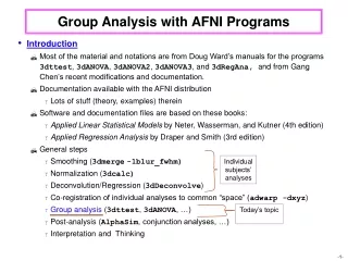
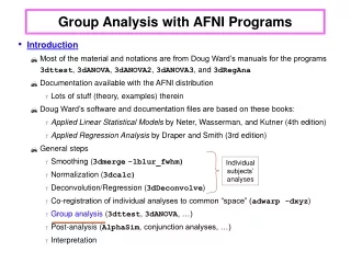
Group Analysis with AFNI Introduction Most of the material and notations are from Doug Ward’s manuals for the programs 3dttest, 3dANOVA, 3dANOVA2, 3dANOVA3, and 3dRegAna Documentation available with the AFNI distribution Lots of stuff (theory, examples) therein Doug Ward’s software and documentation files are based on these books: Applied Linear Statistical Models by Neter, Wasserman and Kutner (4th edition) Applied Regression Analysis by Draper and Smith (3rd edition) General steps Smoothing (3dmerge-1blur_fwhm) Normalization (3dcalc) Deconvolution/Regression (3dDeconvolve) Co-registration (adwarp -dxyz) Group analysis (ANOVA, ANCOVA, …) Post-analysis (AlphaSim, conjunction analysis, …) Interpretation
Data Preparation: Smoothing • Spatial variability of both FMRI and the Talairach transform can result in little or no overlap of function between subjects. • Data smoothing is used to reduce this problem. • Leads to loss of spatial resolution, but that is a price to be paid with the Talairach transform • In principle, smoothing should be done on time series data, before data fitting (i.e., before 3dDeconvolve or 3dNLfim, etc.) • Otherwise one has to decide on how to smooth statistical parameters. • In statistical data sets, each voxel has a multitude of different parameters associated with it like a regression coefficient, t-statistic, F-statistic, etc. • Combining some statistical parameters across voxels might result in parameters with unknown distributions • Blurring is done using 3dmerge with the -1blur_fwhm option • Blurring on the surface is done with program SurfSmooth
Data Preparation: Parameter Normalization • Parameters quantifying activation must be normalized before group comparisons. • FMRI signal amplitude varies for different subjects, runs, scanning sessions, regressors, image reconstruction software, modeling strategies, etc. • Amplitude measures (regression coefficients) can be turned to percent signal change from baseline (do it before individual analysis – 3dDeconvolve). • Equations to use with 3dcalc to calculate percent signal change • 100 bi/ b0 (basic formula) • 100 bi/ b0 * c (mask out the outside of the brain) • bi = coefficient for regressor i (output from 3dDeconvolve) • b0 = baseline estimate (output from 3dTstat -mean) • c = threshold value generated from running 3dAutomask -dilate • Other normalization methods, such as z-score transformations of statistics, can also be used.
Data Preparation: Co-Registration • Group analyses are performed on a voxel-by-voxel basis • All data sets used in the analysis must be aligned and defined over the same spatial domain. • Talairach domain for volumetric data • Landmarks for the transform are set on high-res. anatomical data using AFNI (http://afni.nimh.nih.gov/afni/edu/afni08.pdf) • Functional data volumes are then transformed using AFNI interactively or adwarp from command line (use option -dxyz with same resolution as EPI data) • Standard meshes and spherical coordinate system for surface data • Surface models of the cortical surface are warped to match a template surface using Caret/SureFit (http://brainmap.wustl.edu) or FreeSurfer (http://surfer.nmr.mgh.harvard.edu) • Standard-mesh surface models are then created with SUMA (http://afni.nimh.nih.gov/ssc/ziad/SUMA) to allow for node-based group analysis using AFNI’s programs • Analysis is carried out voxel-by-voxel or node-by-node
Statistical Testing with AFNI • Parametric Tests: • Assume data are normally distributed (Gaussian) • 3dttest (paired, unpaired) • 3dANOVA (or 3dANOVA2 or 3dANOVA3) • 3dRegAna (regression, unbalanced ANOVA, ANCOVA) • Matlab script for one- up to four-way ANOVA (still under development) • Non-parametric analyses: • No assumption of normality • Tends to be less sensitive to outliers (more robust) • 3dWilcoxon (~t-test paired) • 3dMannWhitney (~t-test unpaired) • 3dKruskalWallis (~3dANOVA) • 3dFriedman (~3dANOVA2) • Permutation test • Less sensitive than parametric tests • In practice, seems to make little difference • Probably because number of datasets is usually small
t-Test [starting easy] • Program 3dttest • Used to test if the mean of a set of values is significantly different from a constant (usually 0) or the mean of another set of values. • Assumptions • Values in each set are normally distributed • Equal variance in both sets • Values in each set are independent unpaired t-test • Values in each set are dependent paired t-test • Example: 20 subjects are tested for the effects of 2 drugs A and B • Case 1: 10 subjects were given drug A and the other 10 drug B. • Unpaired t-test is used to test if mA = mB • Equivalent to one-way ANOVA with between-subjects design of equal sample size can also run 3dANOVA • Case 2: 20 subjects were given both drugs at different times. • Paired t-test is used to test if mA = mB • Case 3: 20 subjects were given drug A. • t-test is used to test if drug effect is significant at group level: mA= 0
One-Way ANOVA • Program 3dANOVA • Determine whether treatments (levels) of a factor(independent parameter) has an effect on the measured response (dependent parameter, like percent signal change due to some stimulus). • Examples of factor: task difficulty, drug type, drug dosage, etc. • For fixed effect only • Assumptions • Values are normally distributed • No assumptions about relationship between dependent and independent variables (e.g., not necessarily linear) • Independent variables are qualitative • Can also run 3dttest if there are only two groups with same sample size • Example: Subjects performed a task while taking different doses of a drug
Null Hypothesis: H0 :m1 = m2 = … = mr i.e. drug dose has no effect Alternative Hypothesis: Ha: not all m are equal i.e. at least one drug dose had an effect NOTE: 3dANOVA only allows fixed effect modeling. This means that the inferences about drug dose effect are limited to the doses tested. Effectively, this is a generalization of t-test to multiple columns of data.
ANOVA: Which level had an effect? • which treatment means (mi) are ≠ 0 ? • i.e. is the response to drug dose 3 different from 0? • t-statistic with option -mean in 3dANOVA • Equivalent to using 3dttest -base1 0 when there are only 2 levels with same sample size • which treatment means are different from each other ? • i.e. is the response to drug dose 2 different from the response to dose 3 ? • t-statistic with option -diff in 3dANOVA • Equivalent to using 3dttest (unpaired) when there are only 2 levels with same sample size • which linear combination of means (contrasts) are ≠ 0 ? • i.e. is the response to drug doses 1 and 2 different from the response to drug doses 3 and 4? • t-statistic with option -contr in 3dANOVA
Two-Way ANOVA • Purpose: To test for the effects of two factors on the measurements • i.e., drug type for factor 1 and drug dosage for factor 2 • or drug dosage for factor 1 and subject for factor 2 • Same statistics as one way ANOVA for each of the 2 factors • factor effect • factor mean, difference and contrasts • Statistics for factor interactions • when the effect of factor A depends on the level of factor B and vice-versa • Options for using fixed, random and mixed effect models • Fixed models: • Testing for differences in means between factors • Hypothesis testing applies only to treatments explicitly considered. • i.e. if dose levels of 5 mg, 15 mg and 25 mg are used for treatments, we cannot make a statement about effects of dose levels of 2 mg or 100 mg
Random models: • Testing for differences in variances between factors • Considers levels of the random factor as a random sample from a larger population. Hypothesis testing of the random effect can thus be extended to entire population. • Obviously, one cannot always use random effect model (consider the ‘drug type’ factor) • Subjects are often used as a random factor • Random model tests yield lower F-statistics (less statistical power) because variance of factor effects is tested against that of both factor means, which is often larger than the error variance used in fixed effects. • This is better expressed in the equations of F-ratios that we avoided using in this presentation • Intermediate effects (mean and variance differences) would be nice • Not a standard statistical formula, and not available in AFNI yet
NOTE WELL: Must have same number of observations in each cell Can use 3dRegAna if you don’t have the same number of values in each cell (program usage is much more complicated)
Tests for main effects • Fixed effects: • Null Hypothesis: Ho :m1. = m2.= … = ma. i.e. drug type (factor A) has no effect on mean response • Null Hypothesis: Ho :m.1 = m.2 = … = m.a i.e. drug dose (factor B) has no effect on mean response • Random effects: • Null Hypothesis: Ho : sA2 = 0 i.e. there is no extra variance caused by drug type (factor A) • Null Hypothesis: Ho : sB2 = 0 i.e. there is no extra variance caused by drug dose (factor B) • Tests for interactions • Null Hypothesis: Ho: mij + m.. - mi.- m.j = 0 for all i,j Each level of factor A affects all levels of B in a similar manner and vice versa. i.e. Drug dose has the same effect regardless of drug type. • Alternative: Ha: mij + m.. - mi.- m.j≠ 0 for some i,j i.e. Drug dose 2 has twice the effect for drug type 3 than for drug type 5 • F-Statistic used to test for main effects and interactions
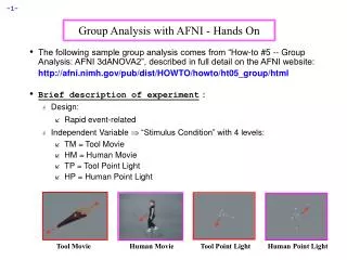
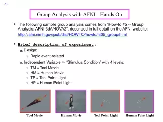
Two-Way ANOVA: Tests on level means • Like with one-way ANOVA, t-statistics are used to test for: • factor level means ≠ 0 • differences of 2 factor level means • Contrast of multiple factor level means • 3dANOVA2: A test case • Michael S. Beauchamp, Kathryn E. Lee, James V. Haxby, and Alex Martin, fMRI Responses to Video and Point-Light Displays of Moving Humans and Manipulable Objects, Journal of Cognitive Neuroscience, 15: 991-1001 (2003). • Purpose is to study the organization of brain responses to different types of complex visual motion • Data from 3 of the subjects, and scripts to process it with AFNI programs, are available in AFNI HowTo #5 (hands-on) • Available for download at the AFNI web site • If you want all the data, it is at the FMRI Data Center at Dartmouth
Tool motion (TM) • Stimuli: Video clips of the following • Human whole-body motion (HM) Human point motion (HP) Tool point motion (TP) From figure 1 Beauchamp et al. 03 • Hypotheses to test: • Which areas are differentially activated by these stimuli (main effect)? • Which areas are differentially activated for point motion versus natural motion (Type of Motion) • Which areas are differentially activated for human versus tool motion (Category of stimulus) • Etc.
Data Processing • IRF for each of the 4 stimuli were obtained using 3dDeconvolve • Regressor coefficients (IRFs) were normalized to percent signal change (using 3dcalc) • An average activation measure was obtained by averaging IRF amplitude from the 4th through the 10th second of the response • Capturing the positive blood-oxygenation level dependent response but not any post-stimulus undershoot. • These activation measures will be the measurements in the ANOVA2 table. • An 3dANOVA2 was carried out with: • Factor A, fixed: HM, TM, HP, TP (the 4 types of stimuli) • Factor B, random: 9 subjects
3dANOVA2 script 3dANOVA2 -type 3 -alevels 4 -blevels 9 \ -dset 1 1 ED+tlrc'[0]' -dset 2 1 ED+tlrc'[1]' \ -dset 3 1 ED+tlrc'[2]' -dset 4 1 ED+tlrc'[3]' \-dset 1 2 EE+tlrc'[0]' -dset 2 2 EE+tlrc'[1]' \ -dset 3 2 EE+tlrc'[2]' -dset 4 2 EE+tlrc'[3]' \ … … -dset 1 9 FN+tlrc'[0]' -dset 2 9 FN+tlrc'[1]' \ -dset 3 9 FN+tlrc'[2]' -dset 4 9 FN+tlrc'[3]' \ -amean 1 TM -amean 2 HM -amean 3 TP -amean 4 HP \ -acontr 1 1 1 1 AllAct \-acontr -1 1 -1 1 HvsT \-acontr 1 1 -1 -1 MvsP \-acontr 0 1 0 -1 HMvsHP \-acontr 1 0 -1 0 TMvsTP \-acontr 0 0 -1 1 HPvsTP \-acontr -1 1 0 0 HMvsTM \-acontr 1 -1 -1 1 Inter \ -fa StimEffect \-bucket AvgANOVA
3dANOVA2: inputs • 3dANOVA2 -type 3 -alevels 4 -blevels 9 \ -dset 1 1 ED+tlrc'[0]' -dset 2 1 ED+tlrc'[1]' \ -dset 3 1 ED+tlrc'[2]' -dset 4 1 ED+tlrc'[3]' \ -dset 1 2 EE+tlrc'[0]' -dset 2 2 EE+tlrc'[1]' \ -dset 3 2 EE+tlrc'[2]' -dset 4 2 EE+tlrc'[3]' \ … … -dset 1 9 FN+tlrc'[0]' -dset 2 9 FN+tlrc'[1]' \ -dset 3 9 FN+tlrc'[2]' -dset 4 9 FN+tlrc'[3]' \
3dANOVA2: stats to output 3dANOVA2 -type 3 -alevels 4 -blevels 9 \ -amean 1 TM -amean 2 HM -amean 3 TP -amean 4 HP \ -acontr 1 1 1 1 AllAct \-acontr -1 1 -1 1 HvsT \-acontr 1 1 -1 -1 MvsP \-acontr 0 1 0 -1 HMvsHP \-acontr 1 0 -1 0 TMvsTP \-acontr 0 0 -1 1 HPvsTP \-acontr -1 1 0 0 HMvsTM \-acontr 1 -1 -1 1 Inter \ -fa StimEffect \-bucket AvgANOVA • -amean 1 TM: estimate mean of factor A, level 1 and label it TM • -acontr : specifies contrast matrix and label 1 1 1 1: all of factor A's levels combined = 0? -1 1 -1 1: contrast between human and tools (HM + HP) - (TM + TP) 1 1 -1 -1: contrast between motion and points (HM + TM) - (HP + TP) 0 1 0 -1: contrast between human motion and points (HM - HP) … … • -fa StimEffect: F-statistic for main effect of factor A • -bucket AvgANOVA: prefix of output data set containing stats
3dANOVA2: viewing results • Main effect: Regions showing difference in activation due to changes in stimulus type • view StimEffect sub-bricks for function and threshold (F-stat = 15, p =10-5) • Factor Means: Activation in response to each category • view TM, HM, etc. sub-bricks (t-stat = 10.6, p = 10-10) • all categories appear to activate same areas • Choose AllAct sub-bricks for finding regions activated by at least one of the stimuli • this region of activation is often used to select an ROI which is examined for subtle effects • Choose HvsT (human versus tools) sub-bricks • note small range of t-values (subtle effects, if any) • lower t-stat threshold to 4, p ~ 5x10⁻⁴ • might want to restrict hypothesis testing to region activated by stimuli • Look for interactions that might complicate your fairy tale • view the Inter sub-bricks to determine if some areas for which the contrast ( TM + HP ) – ( HM + TP ) is significant. • Hopefully you’ll find none, or be prepared to explain it.
Three-WAY ANOVA: 3dANOVA3 • Read the manual first and understand what options are available. • Think long and hard about your inferences and how you’ll manage the interactions. • Do that before you collect the data! • Consider collapsing one factor into another so you can use two-way ANOVA (usually with the cost of less sensitive results). • Four-Way ANOVA: at the door! • Interactive mode in Matlab script • Can run both crossed and nested (i.e. subject nested into gender) design • Heavy duty computation: expect to take minutes to hours • Same script for ANOVA, ANOVA2, and ANOVA3 • Includes contrast tests across all factors • Will try to implement more options such as ANCOVA (ANOVA plus regression with continuous covariates), unbalanced design, missing data, etc. alternative but more user-friendly approach to running 3dRegAna for ANCOVA or unbalanced design.
Regression Analysis: 3dRegAna • Simple linear regression: • Y = b0 + b1X1,+ e • where Y represents the FMRI measurement (i.e. percent signal change) and X is the independent variable (i.e. drug dose) • Multiple linear regression: • Y = b0 + b1X1 + b2X2 + b3X3 + …+ e • Regression with qualitative and quantitative variables (ANCOVA) • i.e. drug dose (5mg, 12mg, 23mg, etc.) is quantitative while drug type (Nicotine, THC, Cocaine) or age group (young vs old) or genotype is qualitative, and usually called dummy (or indicator) variable • 2-way ANOVA and 3-way ANOVA with unequal sample size (with “indicator” variables) • Polynomial regression: • Y = b0 + b1X1 + b2X12 + … + e • Linear regression: model is a linear function of its unknowns bi NOT its independent variables Xi • Not for fitting time series, use 3dDeconvolve (or 3dNLfim) instead
F-test for Lack of Fit (lof) • If repeated measurements are available (and they should be), a Lack Of Fit (lof) test is first carried out. • Hypothesis: H0: E(Y) = b0 + b1X1 + b2X2 + …,+ bp-1Xp-1 Ha: E(Y) ≠b0 + b1X1 + b2X2 + …,+ bp-1Xp-1 • Hypothesis is tested by comparing the variance of the model’s lack of fit to the measurement variance at each point (pure error). • If Flof is significantthen model is inadequate. STOP HERE. • Reconsider independent variables, try again. • If Flof is insignificant then model appears adequate, so far. • It is important to test for the lack of fit: • The remainder of the analysis assumes an adequate model is used • You will not be visually inspecting the goodness of the fit for thousands of voxels!
Test for Significance of Linear Regression • This is done by testing whether additional parameters significantly improve the fit • For simple case Y = b0 + b1X1 + e H0: b1 = 0 H1: b1≠ 0 • For general case Y =b0 + b1X1 + b2X2 + …,+ bq-1Xq-1 + bqXq + … + bp-1Xp-1 + e H0: bq = bq+1 = ... = bp-1 = 0 Ha: bk≠ 0, for some k, q ≤ k ≤ p-1 • Freg is the F-statistic for determining if Full model significantly improved on the reduced model • NOTE: This F-statistic is assumed to have a central F-distribution. This is not the case when there is a lack of fit
3dRegAna: Other statistics • How well does model fit data? • R2 (coefficient of multiple determination) is the proportion of the variance in the data accounted for by the model 0 ≤ R2≤ 1. • i.e. if R2 = 0.26 then 26% of the data’s variation about their mean is accounted for by the model. So this might indicate the model, while significant might not be that useful. • Having said that, you should consider R2 relative to the maximum it can achieve given the pure error which cannot be modeled. [read Draper & Smith, chapter 2]. • Are individual parameters bk significant? • t-statistic is calculated for each parameter • helps identify parameters that can be discarded to simplify the model • R2 and t-statistic are computed for full (not reduced) model
Examples from Applied Regression Analysis by Draper and Smith (third edition)
3dRegAna: Qualitative Variables (ANCOVA) • Qualitative variables can also be used • i.e. We’re modeling the response amplitude to a stimulus of varying contrast when subjects are either young, middle-aged or old. • X1 represents the stimulus contrast (quantitative): covariate • Create indicator variables X2 and X3 to represent age: • X2 = 1 if subject is middle-aged = 0 otherwise • X3 = 1 if subject is old (i.e. at least 1 year older than Bob) = 0 otherwise • Full Model (no interactions between age and contrast) • Y = b0 + b1X1 + b2X2,+ b3X3 + e • E(Y) = b0 + b1X1 for young subjects • E(Y) = ( b0 + b2 )+ b1X1 for middle-aged subjects • E(Y) = ( b0 + b3 )+ b1X1 for old subjects • Full Model (with interactions between age and contrast) • Y = b0 + b1X1,+ b2X2 + b3X3,+ b4X2,X1 + b5X3X1,+ e • E(Y) = b0 + b1X1 for young subjects • E(Y) = ( b0 + b2 )+ ( b1 + b4 )X1 for middle-aged subjects • E(Y) = ( b0 + b3 )+ ( b1 + b5 )X1 for old subjects • Will be available and easier to run analysis in Matlab script
3dRegAna: ANOVA with unequal samples • 3dANOVA2 and 3dANOVA3 do not allow for unequal samples in each combination of factor levels • Can use 3dRegAna to look for main effects and interactions • The analysis method involves the use of indicator variables so it is practical for small for small (~3) factor levels • Details are in the 3dRegAna manual • method is significantly more complicated than running ANOVA; you must understand the math • avoid this, if you can, especially if you have more than 4 factor levels or more than 2 factors • Interactions hard to interpret, and contrast tests unavailable • Will be available and easier to run analysis in Matlab script
Conjunction Junction: What’s Your Function? • The program 3dcalc is a general purpose program for performing logic and arithmetic calculations • command line is of the format 3dcalc -a Dset1 -b Dset2 ... -expr (a * b...) • some expressions can be used to select voxels with values v meeting certain criteria: • find voxels where v > th and mark them with value=1 step (v – th) • in a range of values: thmin < v < thmax step (v – thmin) * step (thmax - v) • exact value: v = n 1 – bool(v – n) • create masks to apply to functional datasets • two values both above threshold: step(v-A)*step(w-B)