Download
1 / 39
410 likes | 441 Vues
Learn group analysis using AFNI with a sample experiment, steps involved, data processing, ANOVA2, and hands-on example to process data efficiently.

E N D
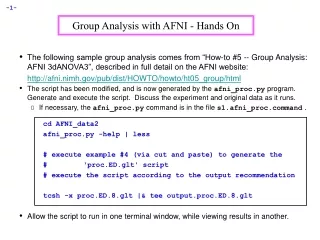
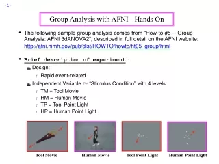
Group Analysis with AFNI - Hands On • The following sample group analysis comes from “How-to #5 -- Group Analysis: AFNI 3dANOVA2”, described in full detail on the AFNI website: http://afni.nimh.gov/pub/dist/HOWTO/howto/ht05_group/html • Brief description of experiment: • Design: • Rapid event-related • Independent Variable “Stimulus Condition” with 4 levels: • TM = Tool Movie • HM = Human Movie • TP = Tool Point Light • HP = Human Point Light Tool Movie Human Movie Tool Point Light Human Point Light
Data Collected: • 1 Anatomical (SPGR) dataset for each subject • 124 sagittal slices • 10 Time Series (EPI) datasets for each subject • 23 axial slices x 138 volumes = 3174 volumes/timepoints per run • note: each run consists of random presentations of rest and all 4 stimulus condition levels • TR = 2 sec; voxel dimensions = 3.75 x 3.75 x 5 mm • Sample size, n=3 (subjects ED, EE, EF) • note: original study had n=10 • Analysis Steps: • Part I: Process data for each subject first • Pre-process subjects’ data many steps involved here… • Run deconvolution analysis on each subject’s dataset --- 3dDeconvolve • Part II: Run group analysis • 2-way Analysis of Variance (ANOVA) --- 3dANOVA2 • i.e., Stimulus Condition (4) x Subjects (3) = 2-way ANOVA
PART I Process Data for each Subject First: • Hands-on example: Subject ED • We will begin with ED’s anat dataset and 10 time-series (3D+time) datasets: EDspgr+orig, EDspgr+tlrc, ED_r1+orig, ED_r2+orig … ED_r10+orig • Below is ED’s ED_r1+orig (3D+time) dataset. Notice the first two time points of the time series have relatively high intensity*. We will need to remove them later: Timepoints 0 and 1 have high intensity values • Images obtained during the first 4-6 seconds of scanning will have much larger intensities than images in the rest of the timeseries, when magnetization (and therefore intensity) has decreased to its steady state value
STEP 1: Volume Register and time shift the voxel time series for each 3D+time dataset using AFNI program3dvolreg • We will also remove the first 2 time points at this step • Use the “foreach” loop to do all 10 of ED’s 3D+time datasets at once: foreach run (1 2 3 4 5 6 7 8 9 10) 3dvolreg -base ED_r{$run}+orig’[2]’ \ -tshift 0 \ -prefix ED_r{$run}_vr \ ED_r{$run}+orig’[2..137]’ end • -base: Timepoint 2 is our base/target volume to which the remaining timepoints (3-137) will be aligned. We are ignoring timepoints 0 and 1 • -tshift 0: For each run, the slices within each volume are being time shifted prior to volume registration. This is done to correct for the different sampling times for each slice • -prefix gives our output files a new name, e.g., ED_r1_vr+orig • ED_r{$run}+orig’[2..137]’ refers to our input datasets (runs 1-10) that will be time shifted and volume registered. Notice that we are removing timepoints 0 and 1
Subject ED’s newly created time shifted and volume registered datasets: ED_r1_vr+orig.HEAD ED_r1_vr+orig.BRIK … … ED_r10_vr+orig.HEAD ED_r10_vr+orig.BRIK • Below is run 1 of ED’s time shifted and volume registered datasets, ED_r1_vr+orig:
STEP 2: Smooth 3D+time datasets with AFNI 3dmerge • The result of spatial blurring (filtering) is somewhat cleaner, more contiguous activation blobs • Spatial blurring will be done on ED’s time shifted, volume registered datasets: foreach run (1 2 3 4 5 6 7 8 9 10) 3dmerge -1blur_rms 4 \ -doall \ -prefix ED_r{$run}_vr_bl \ ED_r{$run}_vr+orig end • -1blur_rms 4 sets the Gaussian filter to have a root mean square deviation of 4mm (You decide the width of the filter) • -doall applies the editing option (in this case the Gaussian filter) to all sub-bricks uniformly in each dataset
Result from 3dmerge: ED_r1_vr+orig ED_r1_vr_bl+orig Before blurring After blurring
STEP 3: Normalizing the Data - Calculating Percent Change • This particular step is a bit more involved, because it is comprised of three parts. Each part will be described in detail: • Set all background values (outside of the volume) to zero with 3dAutomask • Do a voxel-by-voxel calculation of the mean intensity value with 3dTstat • Do a voxel-by-voxel calculation of the percent signal change with 3dcalc • Why should we normalize our data? • Normalization becomes an important issue when comparing data across subjects, because baseline/rest states will vary from subject to subject • The amount of activation in response to a stimulus event will also vary from subject to subject • As a result, the baseline Ideal Response Function (IRF) and the stimulus IRF will vary from subject to subject -- we must account for this variability • By converting to percent change, we can compare the activation calibrated with the relative change of signal, instead of the arbitrary baseline of FMRI signal
For example: Subject 1 - Signal in hippocampus goes from 1000 (baseline) to 1050 (stimulus condition) Difference = 50 IRF units Subject 2 - Signal in hippocampus goes from 500 (baseline) to 525 (stimulus condition) Difference = 25 IRF units • Conclusion: • Subject 1 shows twice as much activation in response to the stimulus condition than does Subject 2 --- WRONG!! • If ANOVA were run on these difference scores, the change in baseline from subject to subject would add variance to the analysis • We must control for these differences in baseline across subjects by somehow normalizing the baseline so that a reliable comparison between subjects can be made
Solution: • Compute Percent Signal Change • i.e., by what percent does the Ideal Response Function increase with presentation of the stimulus condition, relative to baseline? • Percent Change Calculation: • If A = Stimulus IRF • If B = Baseline IRF Percent Signal Change = (A/B) * 100%
Subject 1 -- Stimulus (A) = 1050, Baseline (B) = 1000 (1050/1000) * 100% = 105% or 5% increase in IRF • Subject 2 -- Stimulus (A) = 525, Baseline (B) = 500 (525/500) * 100% = 105% or 5% increase in IRF • Conclusion: • Both subjects show a 5% increase in signal change from baseline to stimulus condition • Therefore, no significant difference in signal change between these two subjects
STEP 3A: Ignore any background values in a dataset by creating a mask with 3dAutomask • Values in the background have very low baseline values, which can lead to artificially large percent signal change values. Let’s remove them altogether by creating a mask of our dataset, where values inside the brain are assigned a value of “1” and values outside of the brain (e.g., noise) are assigned a value of “0” • This mask will be used later when the percent signal change in each voxel is calculated. A percent change will be computed only for voxels inside the mask • A mask will be created for each of Subject ED’s time shifted, volume registered, and blurred 3D+time datasets: foreach run (1 2 3 4 5 6 7 8 9 10) 3dAutomask -prefix mask_r{$run} \ ED_r{$run}_vr_bl+orig end • Output of 3dAutomask: A mask dataset for each 3D+time dataset: mask_r1+orig, mask_r2+orig … mask_r10+orig
Now let’s take those 10 masks (we don’t need 10 separate masks) and combine them to make one master or “full mask”, which will be used to calculate the percent signal change only for values inside the mask (i.e., inside the brain). • 3dcalc -- one of the most versatile AFNI programs -- is used to combine the 10 masks into one: 3dcalc-a mask_r1+orig -b mask_r2+orig -c mask_r3+orig \ -d mask_r4+orig -e mask_r5+orig -f mask_r6+orig \ -g mask_r7+orig -h mask_r8+orig -i mask_r9+orig \ -k mask_r10+orig \ -expr ‘step(a+b+c+d+e+f+g+h+i+j)’ \ -prefix full_mask • Output: full_mask+orig:
STEP 3B: Create a voxel-by-voxel mean for each timeseries dataset with 3dTstat • For each voxel, add the intensity values of the 136 time points and divide by 136 • The resulting mean will be inserted into the “B” slot of our percent signal change equation (A/B*100%) foreach run (1 2 3 4 5 6 7 8 9 10) 3dTstat -prefix mean_r{$run} \ ED_r{$run}_vr_bl+orig end • Unless otherwise specified, the default statistic for 3dTstat is to compute a voxel-by-voxel mean • Other statistics run by 3dTstat include a voxel-by-voxel standard deviation, slope, median, etc…
The end result will be a dataset consisting of a single mean value in each voxel. Below is a graph of a 3x3 voxel matrix from subject ED’s dataset mean_r1+orig: ED_r1_vr_bl+orig Timept 0: 1530 + TP 1: 1515 + TP 2: 1498 + TP … + TP 135: 1522 Divide sum by 136 mean_r1+orig Mean = 1523.346
STEP 3C: Calculate a voxel-by-voxel percent signal change with 3dcalc • Take the 136 intensity values within each voxel, divide each one by the mean intensity value for that voxel (that we calculated in Step 3B), and multiply by 100 to get a percent signal change at each timepoint • This is where the A/B*100 equation comes into play foreach run (1 2 3 4 5 6 7 8 9 10) 3dcalc -a ED_r1_vr_bl+orig \ -b mean_r{$run}+orig \ -c full_mask+orig \ -expr “(a/b * 100) * c” \ -prefix scaled_r{$run} \ end • Output of 3dcalc: 10 normalized datasets for Subject ED, where the signal intensity value at each timepoint has now been replaced with a percent signal change value scaled_r1+orig, scaled_r2+orig …scaled_r10+orig
scaled_r1+orig • E.g., Timepoint #18 above shows a percent signal change value of 101.7501 • i.e., relative to the baseline (of 100), the stimulus presentation (and noise too) resulted in a percent signal change of 1.7501% at that specific timepoint Timepoint #18 Displays the timepoint highlighted in center voxel and its percent signal change value Shows index coordinates for highlighted voxel
STEP 4: Concatenate ED’s 10 normalized datasets into onebig dataset with 3dTcat 3dTcat -prefix ED_all_runs \ scaled_r1+orig \ scaled_r2+orig \ scaled_r3+orig \ scaled_r4+orig \ scaled_r5+orig \ scaled_r6+orig \ scaled_r7+orig \ scaled_r8+orig \ scaled_r9+orig \ scaled_r10+orig \ • The output from 3dTcat is one big dataset -- ED_all_runs+orig -- which consists of 1360 volumes (i.e., 10 runs x 136 timepoints). Every voxel in this large dataset contains percent signal change values • This output file will be inserted into the3dDeconvolve program
STEP 5: Perform a deconvolution analysis on Subject ED’s data with 3dDeconvolve • What is the difference between regular linear regression and deconvolution analysis? • With linear regression, the hemodynamic response is already assumed (we can get a fixed hemodynamic model by running the AFNI waver program) • With deconvolution analysis, the hemodynamic response is not assumed. Instead, it is computed by3dDeconvolve from the data • Once the HRF is modeled by 3dDeconvolve, the program then runs a linear regression on the data • To compute the hemodynamic response function with 3dDeconvolve, we include the “minlag” and “maxlag” options on the command line • The user (you) must determine the lag time of an input stimulus • 1 lag = 1 TR = 2 seconds • In this example, the lag time of the input stimulus has been determined to be about 15 lags • As such, we will add a “minlag” of 0 and a “maxlag” of 14 in our 3dDeconvolve command
3dDeconvolve -input ED_all_runs+orig -num_stimts 4 -stim_file 1 all_stims.1D’[0]’ -stim_label 1 ToolMovie \ -stim_minlag 1 0 -stim_maxlag 1 14 -stim_nptr 1 2 \ -stim_file 2 all_stims.1D’[1]’ -stim_label 2 HumanMovie \ -stim_minlag 2 0 -stim_maxlag 2 14 -stim_nptr 2 2 \ -stim_file 3 all_stims.1D’[2]’ -stim_label 3 ToolPoint \ -stim_minlag 3 0 -stim_maxlag 3 14 -stim_nptr 3 2 \ -stim_file 4 all_stims.1D’[3]’ -stim_label 4 HumanPoint \ -stim_minlag 4 0 -stim_maxlag 4 14 -stim_nptr 4 2 \ -glt 4 contrast1.1D -glt_label 1 FullF \ -glt 1 contrast2.1D -glt_label 2 HvsT \ -glt 1 contrast2.1D -glt_label 3 MvsP \ -glt 1 contrast2.1D -glt_label 4 HMvsHP \ -glt 1 contrast2.1D -glt_label 5 TMvsTP \ -glt 1 contrast2.1D -glt_label 6 HPvsTP \ -glt 1 contrast2.1D -glt_label 7 HMvsTM \ -iresp 1 TMirf -iresp 2 HMirf -iresp 3 TPirf -iresp 4 HPirf \ -full_first -fout -tout -nobout -polort 2 \ -concat runs.1D \ -progress 1000 \ -bucket ED_func
-iresp 1 TMirf • -iresp 2 HMirf • -iresp 3 TPirf • -iresp 4 HPirf • These output files are important because they contain the estimated Impulse Response Function for each stimulus type • The percent signal change is shown at each time lag • Below is the estimated IRF for Subject ED’s “Human Movies” (HM) condition: HMirf+orig
Focusing on a single voxel (from ED’s HMirf+orig dataset), we can see that the IRF is made up of 15 time lags (0-14). Recall that this lag duration was determined in the 3dDeconvolve command • Each time lag consists of a percent signal change value:
To run an ANOVA, only one data point can exist in each voxel • As such, the percent signal change values in the 15 lags must be averaged • In the voxel displayed below, the mean percent signal change =1.557% Mean % sig. chg,. (lags 0-14) = 1.557%
Before averaging the values in each voxel, one option is to remove any “uninteresting” time lags and average only those time lag points that matter • In this example, “uninteresting” refers to time lags whose percent signal change value is close to zero • If we included these uninteresting time lags in our mean calculation, they would pull the mean closer to zero, making it more difficult to pick up any statistically significant results in the ANOVA • In this example, the IRF is fairly small from time lags 0-3, but begins to spike up at time lag 4. It peaks at time lag 7, declines at 9, drops sharply by 10, and decreases steadily from there. • Given this information, one option is to compute the mean percent signal change for time lags 4-9 only 7 8 9 6 5 4
If the mean is computed only for time lags 4-9, then mean percent signal change in the voxel below increases dramatically, from 1.557% (all lags) to 3.086%: 4.590% 7 4.056% 8 3.765% 9 3.361% 6 1.996% 5 0.750% 4 Mean % sig. chg,. (lags 4-9) = 3.086%
STEP 5: Compute a voxel-by-voxel mean percent signal change -- including only time lags 4-9 -- with AFNI 3dTstat • The following 3dTstat command will focus only on time lags 4-9, and compute the mean for those lags • This will be done on a voxel-by-voxel basis, and for each IRF dataset, of which we have four: TMirf, HMirf, TPirf, HPirf foreach cond (TM HM TP HP) 3dTstat -prefix ED_{$cond}_irf_mean \ {$cond}irf+orig’[4..9]’ end
The output from 3dTstat will be four irf_mean datasets, one for each stimulus type. Below are subject ED’s averaged IRF datasets: ED_TM_irf_mean+orig ED_HM_irf_mean+orig ED_TP_irf_mean+orig ED_HP_irf_mean+orig • Each voxel will now contain a single number (i.e., the mean percent signal change). For example: ED_HM_irf_mean+orig
STEP 6: Resample the mean IRF datasets for each subject to the same grid as their Talairached anatomical datasets with adwarp • For statistical comparisons made across subjects, all datasets -- including functional overlays -- should be standardized (e.g., Talairach format) to control for variability in brain shape and size foreach cond (TM HM TP HP) adwarp -apar EDspgr+tlrc \ -dpar ED_{$cond}_irf_mean+orig \ end • The output of adwarp will be four Talairach transformed IRF datasets. ED_TM_irf_mean+tlrc ED_HM_irf_mean+tlrc ED_TP_irf_mean+tlrc ED_HP_irf_mean+tlrc • We are now done with Part 1-- Process Individual Subjects’ Data -- for Subject ED • Go back and follow the same steps for Subjects EE and EF • We can now move on to Part 2 -- RUN GROUP ANALYSIS (ANOVA)
PART 2 Run Group Analysis (ANOVA2): • In our sample experiment, we have two factors (or Independent Variables) for our analysis of variance: “Stimulus Condition” and “Subjects” • IV 1: STIMULUS CONDITION 4 levels • Tool Movies (TM) • Human Movies (HM) • Tool Points (TP) • Human Points (HP) • IV 2: SUBJECTS 3 levels • Subject ED • Subject EE • Subject EF • The mean IRF datasets from each subject will be needed for the ANOVA: ED_TM_irf_mean+tlrcEE_TM_irf_mean+tlrcEF_TM_irf_mean+tlrc ED_HM_irf_mean+tlrcEE_HM_irf_mean+tlrcEF_HM_irf_mean+tlrc ED_TP_irf_mean+tlrcEE_TP_irf_mean+tlrcEF_TP_irf_mean+tlrc ED_HP_irf_mean+tlrcEE_HP_irf_mean+tlrcEF_HP_irf_mean+tlrc
3dANOVA2 -type 3 -alevels 4 -blevels 3 \ -dset 1 1 ED_TM_irf_mean+tlrc \ -dset 2 1 ED_HM_irf_mean+tlrc \ -dset 3 1 ED_TP_irf_mean+tlrc \ -dset 4 1 ED_HP_irf_mean+tlrc \ -dset 1 2 EE_TM_irf_mean+tlrc \ -dset 2 2 EE_HM_irf_mean+tlrc \ -dset 3 2 EE_TP_irf_mean+tlrc \ -dset 4 2 EE_HP_irf_mean+tlrc \ -dset 1 3 EF_TM_irf_mean+tlrc \ -dset 2 3 EF_HM_irf_mean+tlrc \ -dset 3 3 EF_TP_irf_mean+tlrc \ -dset 4 3 EF_HP_irf_mean+tlrc \ -amean 1 TM \ -amean 2 HM \ -amean 3 TP \ -amean 4 HP \ Continued on next page…
-acontr 1 1 1 1 AllAct \ -acontr -1 1 -1 1 HvsT \ -acontr 1 1 -1 -1 MvsP \ -acontr 0 1 0 -1 HMvsHP \ -acontr 1 0 -1 0 TMvsTP \ -acontr 0 0 1 -1 TPvsHP \ -acontr -1 1 0 0 TMvsHM \ -fa StimEffect \ -bucket AvgANOVAv1
Explanation of 3dANOVA2 options: • -type 3: Tells 3dANOVA2 what type of ANOVA model is to be used. Type 3 refers to a mixed effects model (a = fixed, b=random) • Type 1 = fixed effects model (a and b are fixed) • Type 2 = random effects model (a and b are random) • -alevels 4: Our first IV “Stimulus Condition” has 4 levels -- TM,HM,TP,HP • -blevels 3: Our second IV “Subjects” has 3 levels -- ED, EE, EF • -dset a b filename: Sets up all the factor level combinations • For example: Subject (b) EDEEEF TM 1,11,21,3 Stim Cond (a)HM 2,12,22,3 TP 3,13,23,3 HP 4,14,24,3
-amean: Estimates the mean for every level of factor ‘a’ (collapsed across factor ‘b’) and provides a t-statistic for the null hypothesis, Ho: mean = 0 • In this example, the mean percent signal change for each stimulus condition type is averaged across subjects on a voxel-by-voxel basis • For example: Mean Percent Signal Change at Voxel “x” Subject (b) EDEEEF TM 4.1% 3.8% 4.5% M= 4.13% Stim Cond (a)HM 3.2% 2.5% 2.8% M= 2.83% TP 4.6% 4.1% 4.9% M= 4.53% HP 1.7% 2.0% 1.1% M= 1.60% • Allows you to determine if the percent signal change in a voxel is significantly different from zero. If so, appears as colored activation blobs
In class -- Let’s run the ANOVA together: • cd AFNI_data2/group_data • the group_data/ directory contains a script called @anova2 that will run 3dANOVA2 • This script can be viewed with a text editor, e.g., emacs @anova2 • ./@anova2 • execute the ANOVA script from the command line • ls • result from ANOVA script is a bucket dataset AvgANOVAv1+tlrc, stored in the group_data/ directory • afni & • launch AFNI to view the results • The output from 3dANOVA2 is bucket dataset AvgANOVAv1+tlrc, which contains 24 sub-bricks of data: • i.e., means and t-tests for each level of factor A (i.e., “Stimulus Condition”), contrasts between the different levels of factor A, and a main effect of factor A
Brain areas corresponding to “Human Movies” • -amean 2 HM ULay: sample_anat+tlrc OLay: AvgANOVAv1+tlrc Activated areas show percent signal changes -- collapsed across subjects -- that are significantly greater than zero when Human Movies are presented
-acontr: Estimates contrasts among levels of factor ‘a’ • E.g., t-tests are conducted among levels of the factor “Stimulus Condition” to determine if their percent signal changes differ significantly from each other throughout the brain • Here are some contrasts we performed: TMHMTPHPvoxel-by-voxel t-tests: 0 1 0 -1 Human Movies vs. Human Points 1 0 -1 0 Tool Movies vs. Tool Points 0 0 1 -1 Tool Points vs. Human Points 1-1 0 0 Tool Movies vs. Human Movies -11-11 Tools vs. Humans 11-1-1 Movies vs. Points • For simple contrasts, you could also use the -adiff option (e.g., -adiff 2 4) • Tools vs. Humans contrast collapses across Animation Type (i.e., Movies and Points) • Movies vs. Points contrast collapses across Object Type (i.e., Tools and Humans)
Brain areas corresponding to “Movies” (reds) vs. “Point-light displays” (blues) • -acontr 1 1 -1 -1 ULay: sample_anat+tlrc OLay: AvgANOVAv1+tlrc Red blobs show statistically significant percent signal changes in response to “Movies.” Blue blobs show significant percent signal changes in response to “Point-light” displays
-fa: Produces a main effect for factor ‘a’ • In this example, -fa determines which voxels show a percent signal change that is significantly different from zero when any level of factor “Stimulus Condition” is presented • -fa StimEffect: ULay: sample_anat+tlrc OLay: AvgANOVAv1+tlrc Activated areas respond to motion stimuli in general
Many thanks to Mike Beauchamp for donating the data used in this lecture and in the how-to#5 • For a full review of the experiment described in this lecture, see Beauchamp, M.S., Lee, K.E., Haxby, J.V., & Martin, A. (2003). FMRI responses to video and point-light displays of moving humans and manipulable objects. Journal of Cognitive Neuroscience, 15:7, 991-1001. • For more information on AFNI ANOVA programs, download Doug Ward’s paper on Analysis of Variance for FMRI data, located on the AFNI website at: http//afni.nimh.gov/pub/dist/doc3dANOVA.pdf or 3dANOVA.ps