Group Analysis with AFNI Programs

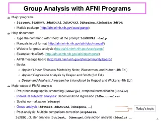
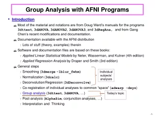
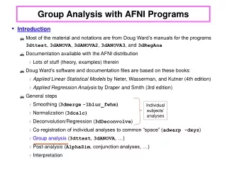
1. Group Analysis with AFNI Programs Major programs 3dttest, 3dANOVA, 3dANOVA2, 3dANOVA3, 3dRegAna, AlphaSim, 3dFDR Matlab package (http://afni.nimh.nih.gov/sscc/gangc) Help documents Type the command with “-help” at the prompt: 3dANOVA2 -help Manuals in pdf format (http://afni.nimh.nih.gov/afni/doc/manual/) Website for group analysis (http://afni.nimh.nih.gov/sscc/gangc) Example: HowTo#5 (http://afni.nimh.nih.gov/afni/doc/howto/) AFNI message board (http://afni.nimh.nih.gov/afni/community/board/) Books: Applied Linear Statistical Models by Neter, Wasserman, and Kutner (4th Ed.) Applied Regression Analysis by Draper and Smith (3rd Ed.) Design and Analysis: A researcher’s handbook by Keppel and Wickens (4th Ed.) Major steps of FMRI analysis Pre-processing: spatial smoothing (3dmerge), temporal normalization (3dcalc) Individual subjects’ analyses: Deconvolution/Regression (3dDeconvolve) Spatial normalization (adwarp) Group analysis (3dttest, 3dANOVA2, 3dRegAna, …) Post-analysis: Multiple comparison correction (AlphaSim, 3dFDR), cluster analysis (3dclust, 3dmerge), conjunction analysis (3dcalc), … Today’s topic

2. Data Preparation I: Spatial Smoothing • Purposes – reduce noise and improve sensitivity: Spatial variability of fMRI activation and the Talairach transform can result in little or no overlap of function across subjects • Mechanism: convolution - weighted average among neighboring voxels • How much? Kernel size usually on the order of 2 voxels • Not sure? Try and compare several different kernel sizes • Downside: Loss of spatial resolution, specificity, and power, but a price to be paid with inter-subject anatomical alignments • Beforeorafter? • Usually done on time series before individual subject analysis • Comparable to group analysis results • Alternatively smooth coefficients/contrasts after individual analysis • Only coefficients (% signal changes) are carried over to group analysis • Programs • Volume data: 3dmerge with the -1blur_fwhm option • Surface data: SurfSmooth

3. Data Preparation II: Parameter Normalization • Parameters quantifying activation must be normalized before group comparisons. • Signal amplitude varies for different subjects, runs, scanning sessions, regressors, image reconstruction software, modeling strategies, etc. • Only meaningful to compare dimensionless numbers: percent signal change • Beforeorafter? • Normalize (scale) before individual subject analysis with 3dcalc: 100 si/ bi * c • si = signal for i-th run • bi = baseline estimate i-th run (output from 3dTstat -mean) • c = multiplier of 1’s or 0’s: mask created with 3dAutomask -dilate • Regression (β) coefficients out of 3dDeconvolve: percent signal changes • More convenient for comparisons between individual and group results • Convert to percent signal change after individual subject analysis: 100 β/ b * c • β = coefficient for a regressor (output from 3dDeconvolve) • b= averaged baseline estimate across runs (output from 3dDeconvolve)??? • c = multiplier generated from running 3dAutomask -dilate • Problematic if baselines vary a lot cross runs • Traditionally done before individual subject analysis • Normalize each run separately! • No difference on statistics, and little difference on % signal changes (underestimate) • Cautionary check: baseline constants should be close to (slightly less than) 100

4. Data Preparation III: Data Concatenation • Run and session: difference vague • For sessions (not scanned consecutively), run spatial normalization if concatenation is desirable • Concatenateornot? 3 approaches, 3 purposes • Real concatenation (default): concatenate all runs of data before individual subject analysis • Concatenate all runs, but an event is treated the same across all runs • Normalize before individual subject analysis to avoid cross-run variability of base line • Can’t test cross-run variability • No concatenation: don’t concatenate before individual analysis • Analyze each run with same event modeled separately with 3dDeconvolve • Only possible if there are multiple repeats of an event in each run with similar design across runs • More desirable if variability across runs is big • Test cross-run difference at group level with an extra factor of run • Can’t test cross-run difference at individual level • Pseudo concatenation • Concatenate all runs, but same event is modeled separately for each run • Only possible there are multiple repeats of each event in each run with similar design across runs • More desirable if variability across runs is big • Most flexible: Can test cross-run/session difference in both individual and group analyses, or • Test cross-run/session at individual level, and bring averaged coefficients to group level

5. Data Preparation IV: Co-Registration (AKA “Spatial Normalization”) • Improve sensitivity: Group analysis on voxel-by-voxel basis; Must be aligned/defined over same domain • Beforeorafter? • Usually done after individual subject analysis • Keep close to the original data • Save huge runtime in 3dDeconvolve • Can alternatively done before 3dDeconvolve • More desirable for cross-session concatenation • Compare group results with individual activation maps • Before or after, no significant difference in terms of group analysis results • Convert to lower resolution with roughly the same resolution as EPI (adwarp -dxyz) • Steps and programs • Volumetric data • Anatomical data transformation: manual (AFNI) or automatic (@auto_tlrc) • Transform functional data using AFNI interactively or adwarp (use option -dxyz with about the same resolution as EPI data — do not have to use the default 1 mm resolution!) • Surface data: Standard meshes and spherical coordinate system • Surface models of the cortical surface are warped to match a template surface using Caret/SureFit (http://brainmap.wustl.edu) or FreeSurfer (http://surfer.nmr.mgh.harvard.edu) • Standard-mesh surface models are then created with SUMA (http://afni.nimh.nih.gov/ssc/ziad/SUMA) to allow for node-based group analysis • Once data is aligned, analysis is carried out voxel-by-voxel or node-by-node • Analyses and results are on the percent signal changes • Display resulting statistics (voxel-wise or node-wise) AFNI and/or SUMA

6. Basics about null hypothesis significance testing (NHST) • Controversy: Are humans cognitively good intuitive statisticians? • Quiz: HIV prevalence = 10-3, false + of HIV test = 5%, power of HIV test = 100%. • P(HIV+ | test+) = ? • Cohen, J., "The Earth Is Round (p < .05)“ (1994), American Psychologist, 49, 12 997-1003 • Ritualized dichotomous decisions around a sacred number 0.05 • H0: no task effect or no response difference between two tasks at a voxel vs H1: there is difference • What does it mean with a dichotomous decision and rejecting H0 at a significant level α (e.g., 0.05)? • Conditional probabilityP(result | H0) = α, not P(H0)! • 2 types of errors: type I and type II • Type I error = α, Type II error = β = P(accept H0 | H1); Power = P(accept H1 | H1) = 1 – β • Traditional strategy: control type I error while gaining power as much as possible • Importance of checking efficiency (power) of your design with RSFgen before scanning • Norman H. Anderson: “the main function of statistics is to get more information into the data." • Usual misinterpretations • Reject H0==> Prove or confirm a theory (alternative hypothesis)! (wrong!) • P(result | H0) = P(H0) (wrong!) • P(result | H0) = Probability if the experiment can be reproduced (wrong!) • Keep in mind • Better plan than sorry: Spend more time on experiment design (power analysis) • More appropriate for detection than sanctification of a theory • Try to avoid unnecessary overstatement when making conclusions • Present graphics and report percent signal change, standard deviation, confidence interval, … • Replications are the best strategy on induction/generalization

7. Quiz: How do you interpret the results of a null hypothesis significance test?A researcher tested the null hypothesis that two population means are equal (H0: μ1 = μ2). A t-test produced p=0.01. Assuming that all assumptions of the test have been satisfied, which of the following statements are true and which are false? Why?   1. There is a 1% chance of getting a result even more extreme than the observed one when H0 is true.   2. There is a 1% likelihood that the result happened by chance.   3. There is a 1% chance that the null hypothesis is true.   4. There is a 1% chance that the decision to reject H0 is wrong.   5. There is a 99% chance that the alternative hypothesis is true, given the observed data.   6. A small p value indicates a large effect.   7. Rejection of H0 confirms the alternative hypothesis.   8. Failure to reject H0 means that the two population means are probably equal.   9. Rejecting H0 confirms the quality of the research design.  10. If H0 is not rejected, the study is a failure.  11. If H0 is rejected in Study 1 but not rejected in Study 2, there must be a moderator variable that accounts for the difference between the two studies.  12. There is a 99% chance that a replication study will produce significant results.  13. Assuming H0 is true and the study is repeated many times, 1% of these results will be even more inconsistent with H0 than the observed result.Adapted from Kline, R. B. (2004). Beyond significance testing. Washington, DC: American Psychological Association (pp. 63-69). Dale Berger, CGU 9/04

8. Basics of Group Analysis • General Linear Model (GLM) and ANOVA • Factor and level • Dependant and independent variable • Factors: categorizing variables, e.g., subject category and stimulus class • Levels: nominal (qualitative) values of a factor, e.g., conditions 1, 2, and 3 • Fixed/random factor • Fixed: effects/contrasts at specific levels are of interest • Random (usually subject in fMRI): each level of the factor is not of interest, but should model variance for generalizing the conclusion to whole population • Factorial (crossed)/nested (more specifically within-subject/between-subjects) design • Different terminology • count subject as a random factor (statisticians) • within-subject (repeated measures)/between-subjects (psychologists) • Group analysis: partition/untangle data variability into various sources • Cell-mean (or structural) model of one-way within-subject ANOVA: Yij = μ + αi+ βj + εij • Yij independent variable, percent signal change of subject j with task i; • μ constant – grand/common mean; • αi constants subject to Σαi = 0 – simple effect of factor A at level i, i = 1, 2, ..., a;  • βj independent N(0, σp2) – random effect of subject j, j = 1, 2, ..., b (σp2 - population variance); • εij independent N(0, σ2) – interaction: within-subject variability (σ2 - variance of sampling error)

9. Basics of Group Analysis • Main/simple effect, interaction, and contrast • Main effect: general info regarding a factor • Simple effect: specific info regarding a factor level • Disordinal interaction: differences reverse sign • Ordinal interaction: one above another • Contrast: comparison of 2 or more simple effects; coefficients add up to 0 • Trend analysis: Linear, quadratic or cubic effect • Among stimuli (individual subject analysis) • Among factor levels (group analysis) • If equally-spaced, use the orthogonal polynomial coefficients No. of Conditions/Levels 1 2 3 4 5 6---------------------------------------------------------------------------------------------------------3 Linear -1 0 1 Quadratic 1 -2 1 --------------------------------------------------------------------------------------------------------- Linear -3 -1 1 34 Quadratic 1 -1 -1 1 Cubic -1 3 -3 1--------------------------------------------------------------------------------------------------------- Linear -2 -1 0 1 25 Quadratic 2 -1 -2 -1 2 Cubic -1 2 0 -2 1--------------------------------------------------------------------------------------------------------- Linear -5 -3 -1 1 3 56 Quadratic 5 -1 -4 -4 -1 5 Cubic -5 7 4 -4 -7 5 • If unequally-spaced, contrast coefficients have to be specially constructed Main effects and interactions in 2-way mixed ANOVA

10. Overview of Statistical Testing of Group Datasets with AFNI programs • Non-parametric analysis • No assumption of normality • More appropriate when number of subjects too few • Tend to be less sensitive to outliers (more robust) • Programs: ranking • 3dWilcoxon (~ paired t-test) • 3dMannWhitney (~ two-sample t-test) • 3dKruskalWallis (~3dANOVA) • 3dFriedman (~3dANOVA2) • Permutation test plugin in AFNI under Define Datamode / Plugins / Permutation Test • Can’t run complicated design types • Less sensitive and less flexible than parametric tests

11. Overview of Statistical Testing of Group Datasets with AFNI programs • Parametric Tests • Data normally and independently distributed (Gaussian) and sphericity assumption met • 3dttest (one-sample, unpaired and paired) and 3dANOVA2 (one-way within-subject) • 3dANOVA, 3dANOVA3, 3dRegAna (regression, unbalanced ANOVA, ANCOVA) • Matlab package = script for up to 5-way ANOVA • Sphericity: The roundness of an n-D object • Between-subject factors: homogeneity of variance Heteroscedasticity? usually not too serious • Within-subject factors: homogeneity of level difference variances A little more stringent but easier-to-verify assumption: compound symmetry Tasks A1  A2 A3  A4  A1 s12 s12s13 s14 A2 s21 s22 s23 s24 A3 s31s32 s32 s34 A4 s41 s42 s43 s42 • Compound symmetry: homogeneity of variances; homogeneity of covariances/correlations • Compound symmetry  sphericity; not true the other direction, but rare • How serious is sphericity violation? • Sphericity test (under consideration)

12. Overview of Statistical Testing of Group Datasets with AFNI programs • Parametric Tests • Basic rule to avoid potential sphericity violation: Simple effects and contrasts involving a portion of the data is tested exclusively based on that specific portion • Variance: pooled vs. focused • The following 3 scenarios are immune to sphericity violation: • Simple effect: one-sample t test (3dttest) or one-way within-subject (3dANOVA2) • Contrast: one-sample, paired t test (3dttest) or one-way within-subject (3dANOVA2) • With 2 levels for all factors, no issue of sphericity violation in multi-way ANOVA • Multiple coefficients for each condition (IRF with basis functions including deconvolution) • “Area” Under the Curve (AUC) with t test Simplifying: reduce multiple numbers to one for group H0: Σci = 0 • Take all coefficients to group analysis: A possible new option of F test in 3dANOVA2 H0: c1 = 0, c2 = 0, ..., ck = 0 • Comparisons between the 2 approaches AUC is better: Simple and easy for group analysis, especially important in multi-ANOVA Effect directionality with t test (F doesn’t indicate any direction) Available now in both individual and group analysis Downside of AUC: How to interpret the “area” in cases of other basis functions: tent, gamma, Fourier, etc.? Usually ignore head and tail (undershoot) of IRF Assuming similar shape of IRF across brain and across subjects Bias on some specific interval of IRF: not all coefficients treated equally Both vulnerable to sphericity departure? Homogeneity of correlation: Similarly sequentially-correlated Homogeneity of variance

13. Overview of Statistical Testing of Group Datasets with AFNI programs • Parametric Tests • What are the differences between the two approaches? • Rejection areas slightly different: 2 non-overlapping areas I and III quadrants: smaller p value with AUC (Var(sum)>average Var) II and IV quadrants): bigger p value with AUC (Var(sum)>average Var) Only along the two axes, the 2 approaches match • AUC is good for direction while F-test is better for subtle difference. Ideally run both.

14. t-Test: 3dttest • Student’s t distribution, developed by Gossett, tests if the mean of a set of data is different from a constant (usually 0) or the mean of another set of data. • 3 usages: one-sample, two-sample, and paired t test. • Assumptions • Values in each set are normally distributed with equal variance • Sphericity issue? No issue of sphericity violation • Values in each set are independent? Compare a task between 2 groups:unpairedt-test • Values in each set are dependent? Compare two tasks for one group: pairedt-test • Example: effects of 2 conditions A and B at group level • Case 1: 15 subjects were given condition A • One-samplet test: effect of A is significant at group level μA= 0? • Case 2: 15 subjects under condition A and 13 other subjects under B • Two-samplet test: μA = μB (average response is the same?) • OK with unequal sample sizes • Equivalent to 1-way between-subject ANOVA • Case 3: 15 subjects under both conditions • Pairedt test is used to test: μA = μB? • Equivalent to one-way within-subject (3dANOVA2 -type 3) • Equivalent to run one-sample t test on individual differences/contrasts

15. t-Test: 3dttest • Example: 2-way (2X2) within-subject design (16 subjects) - AXBXC • 4 tasks (word, picture, spoken, sound) categorized as the following: Modality: visual, auditory Format: verbal, nonverbal visual verbal = word, visual nonverbal = picture, auditory verbal = spoken, auditory nonverbal = sound • What is the word or word-picture effect at group level? H0: word = 0, or H0: word-picture = 0 (one-sample t test!) • 3dANOVA3 -type 4 would not work because of lack of 2nd contrast testing option • Can also run GroupAna • Script of paired t test for H0: word-picture = 0 3dttest -prefix Wd-Pic \ -paired \ -set1 Wd_S1+tlrc ... Wd_S16+tlrc \ -set2 Pic_S1+tlrc ... Pic_S16+tlrc \ • Can also run a one-sample t test for H0: word-picture = 0 • Picture/spoken/sound/ or spoken-sound/word-spoken/picture-sound effect? (quiz!) Name of output dataset We want a paired t test Input of first datasets Input of second datasets

16. 1-Way ANOVA: 3dANOVA • Generalization of two-sample t-test • One-way between-subject • Null hypothesis H0: no difference across all the factor levels (groups) • Examples of factor: subject group such as gender, age group, genotype, disease, etc. • OK with unequal sample sizes • Assumptions • Values are normally distributed with equal variances across levels (groups) • Unlike regression analysis, no assumptions about relationship between dependent and independent variables (e.g., not necessarily linear) • Independent variable (e.g., gender, disease, genotype, etc.) is qualitative • 3dANOVA versus 3dttest • Equivalent when there are only two levels • More than 2 levels • Can still run two-sample t-test on paired levels with 3dttest to obtain contrasts • Results should be similar unless there is significant heteroscedasticity across levels • Pooled variance vs. between-levels variance • 3dttestis better if heteroscedasticity is significant across groups

17. Specifies model type, number of levels in factors • 2-Way ANOVA: 3dANOVA2 • 3 design types, most frequently used design: 3dANOVA2 –type 3 (one-way within-subject) • Extension of paired t test • No concern of sphericity violation for simple effect and contrast testing • Example: 3dANOVA2 script 3dANOVA2 -type 3 -alevels 4 -blevels 9 \ -dset 1 1 ED+tlrc'[0]' -dset 2 1 ED+tlrc'[1]' \ -dset 3 1 ED+tlrc'[2]' -dset 4 1 ED+tlrc'[3]' \-dset 1 2 EE+tlrc'[0]' -dset 2 2 EE+tlrc'[1]' \ -dset 3 2 EE+tlrc'[2]' -dset 4 2 EE+tlrc'[3]' \ … … -dset 1 9 FN+tlrc'[0]' -dset 2 9 FN+tlrc'[1]' \ -dset 3 9 FN+tlrc'[2]' -dset 4 9 FN+tlrc'[3]' \ -amean 1 TM -amean 2 HM -amean 3 TP -amean 4 HP \ -acontr 1 1 1 1 AllAct \-acontr -1 1 -1 1 HvsT \-acontr 1 1 -1 -1 MvsP \-acontr 0 1 0 -1 HMvsHP \-acontr 1 0 -1 0 TMvsTP \-acontr 0 0 -1 1 HPvsTP \-acontr -1 1 0 0 HMvsTM \-acontr 1 -1 -1 1 Inter \ -fa StimEffect \ -bucket AvgANOVA Specifies inputs to each cell in ANOVA table: totally 4X9 = 36 combinations Output sub-bricks with simple effect for each A level, equivalent to one-sample t test Specifies contrast tests among various cells, equivalent to paired t test Output sub-brick with factor A “main effect” F test Name of output dataset

18. 3-Way ANOVA: 3dANOVA3 • Most frequently used designs • Type 4 (two-way within-subject) - crossed design (AXBXC): generalization of paired t-test • Type 5 (two-way mixed) - classification factor A can’t be varied within a subject: BXC(A) • Has new concept: nested design (vs. fully crossed design) or between-subjects factor • Nested design: each level of one factor contains a unique set of levels of the other • Example • Design type 5 BXC(A) • factor A = subject type; level #1=wild type P, #2=genotype Q, #3=genotype R • factor B = stimulus type; levels #1–4=different types of tasks • factor C = subject; 30 different subjects, 10 for each genotype; C is “nested” inside A • Mixture of unpaired and paired tests with one between-subject and one within-subject • Paired across stimulus type (factor B) – within-subject (repeated-measures) factor • Unpaired across subject types (factor A levels) - between-subjects • Limitation: no 2nd-order contrasts; balanced design for type 5 (mixed design)  Matlab package GroupAna

19. 4,5-Way ANOVA • Multi-ANOVA • Test for interactions • Difficult to test and interpret simple effects/contrasts • Interactive Matlab script: http://afni.nimh.nih.gov/sscc/gangc • Requires Matlab plus its Statistics Toolbox (pricey) • GLM approach, different from programs 3dANOVAx • Heavy duty computation: minutes to hours • input with lower resolution recommended • use adwarp -dxyz # and 3dresample • Same script can also run 1,2,3-way ANOVA • Includes contrast tests across all factors • Can handle both volume and surface data • Can handle the following unbalanced designs (two-sample t test type): • 3-way ANOVA type 3: BXC(A) • 4-way ANOVA type 3: BXCXD(A) • See http://afni.nimh.nih.gov/sscc/gangc for more info

20. 5 Design Types of 4-Way ANOVA

21. 3 Design Types of 5-Way ANOVA • A real example with 5-way mixed design (neural mechanism for category-selective response): • Factors • Task (between-subject): semantic decision, naming • Modality: visual, auditory • Format: verbal, nonverbal • Category: animal, tool • Subject (random) • 4 stimuli (2X2) for animal and tool - visual verbal = word, visual nonverbal = picture, auditory verbal = spoken, auditory nonverbal = sound • 4-way mixed design: Only 2 levels for all 3 within-subject factors: no sphericity violation

22. >> GroupAna How many factors? 5 Available design types:     Type 1: Factorial (crossed) design AXBXCXDXE - all 5 factors are fixed.     Type 2: Factorial (crossed) design AXBXCXDXE - only factor E is random. If E is subject it is also             called 4-way design with all 4 factors A, B, C and D varying within subject.     Type 3: Mixed design BXCXDXE(A)- only the nested (5th) factor E (usually subject) is random.             Also called 4-way design with factors B, C and D varying within subject and factor A between subjects. Choose design type (1, 2, 3, 4, 5): 3 Is the design balanced? (1 - Yes; 0 - No) 1 Label for No. 1 factor: task How many levels does factor A (task) have? 2 Label for No. 1 level of factor A (task) is: sem Label for No. 2 level of factor A (task) is: nam Label for No. 2 factor: mod How many levels does factor B (mod) have? 2 Label for No. 1 level of factor B (mod) is: vis Label for No. 2 level of factor B (mod) is: aud Label for No. 3 factor: format How many levels does factor C (format) have? 2 Label for No. 1 level of factor C (format) is: dir Label for No. 2 level of factor C (format) is: ind Label for No. 4 factor: cat How many levels does factor D (cat) have? 2 Label for No. 1 level of factor D (cat) is: animal Label for No. 2 level of factor D (cat) is: tool Label for No. 5 factor: subj How many levels does factor E (subj) have? 16 Label for No. 1 level of factor E (subj) is: S1 …… All input files are supposed to contain only one subbrik. There should be totally 256 input files. Correct? (1 - Yes; 0 - No) 1 (1) factor combination:     factor A (task) at level 1 (sem)     factor B (mod) at level 1 (vis)     factor C (format) at level 1 (dir)     factor D (cat) at level 1 (animal)     factor E (subj) at level 1 (S1)     at repeat 1 is: ss03.a_word+tlrc.BRIK

23. …… Output file name (in bucket format): test Any contrast test (1 - Yes, 0 - No)? 1 1st order contrasts have 4 factor(s) collapsed. How many 1st-order contrasts? (0 if none) 4 Label for 1st order contrast No. 1 is: taskdiff How many terms are involved? 2 Factor index for No. 1 term is (e.g., 00200): 10000 Corresponding coefficient (e.g., 1 or -1): 1 Factor index for No. 2 term is (e.g., 00200): 20000 Corresponding coefficient (e.g., 1 or -1): -1…… How many 2nd-order contrasts? (0 if none) 21 Label for 2nd order contrast No. 1 is: avt1 How many terms are involved? 2 Factor index for No. 1 term is (e.g., 01200): 10010 Corresponding coefficient (e.g., 1 or -1): 1 Factor index for No. 2 term is (e.g., 01200): 10020 Corresponding coefficient (e.g., 1 or -1): -1……How many 4th-order contrasts? (0 if none) 9 Label for 4th order contrast No. 1 is: word_avt1 How many terms are involved? 2 Factor index for No. 1 term is (e.g., 01230): 11110 Corresponding coefficient (e.g., 1 or -1): 1 Factor index for No. 2 term is (e.g., 01230): 11120 Corresponding coefficient (e.g., 1 or -1): -1…… Total slices along Z axis: 37. Running analysis on slice: #1... done in 40.940792 seconds ……#37... done in 49.008655 seconds Congratulations, job is done!!! Total runtime: 41.528963 minutes... Output files are test+tlrc.*

24. ANCOVA: Analysis of Covariance • Subjects might not be an ideally randomized representation of a group • Such uncontrollable variables called covariates • Typical covariates in fMRI: age, behavioral data (response time), cortex thickness, … • If no controlled, analysis would be confounded by those covariates • Indirect (statistical) control by untangling covariate effect: ANCOVA = Regression + ANOVA • Assumption: Linear relation between percent signal change and the covariate • Try to avoid multi-way ANCOVA and analyze partial data with a simple one-way ANCOVA • Counterpart of a one-sample or two-sample t test • Centralize your covariate first so that it would not confound with other effects • Example: Running ANCOVA • Two groups: 15 normal vs. 13 patients • Model Yi = β0 + β1X1i + β2X2i +β3X3i +εi, i = 1, 2, ..., n • Remove the mean from the covariate X1 first! • Code the factor (group) with a dummy variable             0, when the subject is a patient; X2i = {              1, when the subject is normal. • If covariate X1 is centralized, β0 reflects the effect of patient group • X3i= X1i X2i models interaction (optional) between covariate and factor (group)

25. Specifies parameters Specifies RAM = 1GB Specifies covariates, factor levels, interaction, and input files • ANCOVA : Analysis of Covariance 3dRegAna -rows 28 -cols 3 \ -workmem 1000 \ -xydata 0.1 0 0 patient/Pat1+tlrc.BRIK \-xydata 7.1 0 0 patient/Pat2+tlrc.BRIK \… -xydata 7.1 0 0 patient/Pat13+tlrc.BRIK \-xydata 2.1 1 2.1 normal/Norm1+tlrc.BRIK \-xydata 2.1 1 2.1 normal/Norm2+tlrc.BRIK \… -xydata -8.9 1 -8.9 normal/Norm14+tlrc.BRIK \-xydata 0.1 1 0.1 normal/Norm15+tlrc.BRIK \ -model 1 2 3 : 0 \ -bucket 0 Pat_vs_Norm \ -brick 0 coef 0 ‘Pat’ \-brick 1 tstat 0 ‘Pat t' \-brick 2 coef 1 'Age Effect' \-brick 3 tstat 1 'Age Effect t' \-brick 4 coef 2 'Norm-Pat' \-brick 5 tstat 2 'Norm-Pat t' \-brick 6 coef 3 'Interaction' \-brick 7 tstat 3 'Interaction t' See http://afni.nimh.nih.gov/sscc/gangc/ANCOVA.html for more information Specifies reduced model for F and R^2 Specifies output format: Total subbriks = 2*#coef + F + R2 Labels output subbriks

26. Multiple comparison correction:AlphaSim • 2 types of errors in statistical tests • What is H0 in FMRI studies? • Type I = P (reject H0|when H0 is true) = false positive = so-called p value Type II = P (accept H0|when H1 is true) = false negative = β (power = 1- β = probability to detect true activation) • Significance level = α: p < α • Dilemma: Usual strategy – controlling type I error (similar to the legal system) • Sex ratio at birth as an example for multiple comparison issue • Almost all statistical analyses in AFNI are done voxel-wise  multiple comparison problem: the increase of the chance that at least one detection is wrong in cluster analysis • 3 occurrences of multiple comparisons: individual, group, and conjunction • Group analysis is the most concerned • For an ROI of nindependent voxels of no activation, the chance to mistakenly label at least one active voxel: αFW = 1-(1- α)n ~ nα αFWbecomes big as n increases • multiple comparison correction - controlling the severity of family-wise error: making αFW reasonably small without losing too much power! • Bonferroni correction: to achieve an overall significance level of α, take α/n as individual significance level  αFW = α • Bonferroni correction is too stringent and overly conservative for FMRI analysis  not many voxels can survive  lose statistical power, failing to detect true activations! • Assumption of independence vs. brain structure

27. Multiple comparison correction:AlphaSim • Monte Carlo simulation: AlphaSim • Named for Monte Carlo, Monaco, where the primary attractions are casinos • Randomly generates values for uncertain variables over and over to simulate a model for data in EPI resolution • Obtain simulated (estimated) overall significance level (corrected p-value) for a minimum cluster size and individual voxel significance level: counterbalance among all 3! • Should be done in original space • General steps • Create mask or ROI  reducing voxel number avoids unnecessary sacrifice and leads to relaxation of cluster threshold; masking always recommended, ROI for small regions such as amygdala • Obtain spatial correlation: number in option -1blur_fwhm of 3dmerge • Calculate connectivity radius: Consider EPI (not tlrc) resolution; e.g., use a number slightly larger than the diagonal length of a voxel • Example: AlphaSim \-mask brain_mask+tlrc \-fwhmx 10 -fwhmy 10 -fwhmz 8 \-rmm 8.1 -pthr 0.005 -iter 1000 \-out AlphaSim_out

28. Multiple (simultaneous) comparison correction:AlphaSim • Output – 5 columns • Cluster size: in voxels • Frequency: number of clusters for a specific cluster size • Cumulative probability • p/Voxel: ignore it! • Maximum frequency: occurrences of maximum cluster with the specified size • Alpha (α): overall significance level (corrected p value) • Example Cl Size Frequency Cum Prop p/Voxel Max Freq Alpha1 1826 0.984897 0.00509459 831 0.859 2 25 0.998382 0.00015946 25 0.028 3 3 1.0 0.00002432 3 0.003

29. False Discovery Rate: 3dFDR • FDR = Nia/Da = Nia/(Naa+ Nia) – proportion of voxels declared as active but truly inactive • Does not consider cluster size and connectivity • Does not control the chance of any false positives • Only controls the expected percent of false positives among declared active voxels • More lenient and sensitive than other correction methods • Algorithm: statistic  p value  FDR (q value)  z score • Example: 3dFDR -input ‘Group+tlrc[6]' \ -mask_file mask+tlrc -mask_thr 1 \ -cdep -list \ -output test • Index p-value q-value z-score 2821453 0.000001 0.004033 2.875584 2852202 0.000003 0.005840 2.756648 2355533 0.001513 0.564017 0.576886 ……

30. Conjunction Analysis: What’s Your Function? • 3dcalc: a general purpose program for performing logic and arithmetic calculations • Command line is of the format 3dcalc -a Dset1 -b Dset2 ... -expr “(a * b ...)” • The Heaviside Unit Step Function defines functions encountering ideal On/Off: values from Dset1 are to be called ‘a’ in -expr mathematical expression combining input dataset values

31. Conjunction Analysis: What’s Your Function? • Some expressions can be used to select voxels with values v meeting certain criteria: • Find voxels where v th and mark them with value=1expression =step (v – th) • In a range of values: thmin≤ v ≤ thmaxexpression =step (v – thmin) * step (thmax - v) • Exact value: v = n expression =equals(v – n) • Create masks to apply to statistical (t or F) subbriks • Two values both above threshold(e.g. “conjunction”)expression =step(v-A)*step(w-B) • Example of conjunction analysis with 3 contrasts: A vs D, B vs D, and C vs D • Map 3 contrasts to 3 numbers: A > D: 1; B > D: 2; C > D: 4 • Create a mask with 3 tstatistical subbriks (with t threshold of 4.2): 3dcalc -a func+tlrc'[5]' -b func+tlrc'[10]' -c func+tlrc'[15]‘ -expr 'step(a-4)+2*step(b-4)+4*step(c-4)' -prefix cond_mask • 23 = 8 possible combinations: 0 – none; 1 - A > D but no others; 2 - B > D but no others; 3 - A > D and B > D but not C > D; 4 - C > D but no others; 5 - A > D and C > D but not B > D; 6 - B > D and C > D but not A > D; 7 – all 3 contrasts