Group Analysis with AFNI Programs

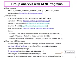
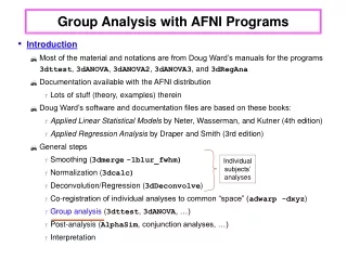
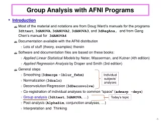
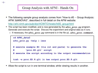
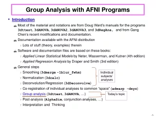
1. Group Analysis with AFNI Programs Introduction Most of the material and notations are from Doug Ward’s manuals for the programs 3dttest, 3dANOVA, 3dANOVA2, 3dANOVA3, and 3dRegAna, and from Gang Chen’s recent modifications and documentation. Documentation available with the AFNI distribution Lots of stuff (theory, examples) therein Software and documentation files are based on these books: Applied Linear Statistical Models by Neter, Wasserman, and Kutner (4th edition) Applied Regression Analysis by Draper and Smith (3rd edition) General steps Smoothing (3dmerge-1blur_fwhm) Normalization (3dcalc) Deconvolution/Regression (3dDeconvolve) Co-registration of individual analyses to common “space” (adwarp -dxyz) Group analysis (3dttest, 3dANOVA, …) Post-analysis (AlphaSim, conjunction analyses, …) Interpretation and Thinking Individual subjects’ analyses Today’s topic

2. Data Preparation: Spatial Smoothing • Spatial variability of both FMRI activation and the Talairach transform (the common space) can result in little or no overlap of function between subjects. • Data smoothing is used to reduce this problem. • Leads to loss of spatial resolution, but that is a price to be paid with the Talairach transform (or any current technique that does inter-subject anatomical alignments) • In principle, smoothing should be done on time series data, before data fitting (i.e., before 3dDeconvolve or 3dNLfim, etc.) • Otherwise one has to decide on how to smooth statistical parameters. • In statistical data sets, each voxel has a multitude of different parameters associated with it like a regression coefficient, t-statistic, F-statistic, etc. • Combining some statistical parameters across voxels would result in parameters with unknown distributions • It is OK to blur percent signal change values that come out of the regression analysis, since these numbers depend linearly on the input data (unlike the F- and t-statistics) • Blurring in 3D is done using 3dmerge with the -1blur_fwhm option • Blurring on the surface is done with program SurfSmooth

3. Data Preparation: Parameter Normalization • Parameters quantifying activation must be normalized before group comparisons. • FMRI signal amplitude varies for different subjects, runs, scanning sessions, regressors, image reconstruction software, modeling strategies, etc. • Amplitude measures (regression coefficients) can be turned to percent signal change from baseline (do it before the individual analysis in 3dDeconvolve). • Equations to use with 3dcalc to calculate percent signal change • 100 bi/ b0 (basic formula) • 100 bi/ b0 * c (mask out the outside of the brain) • bi = coefficient for regressor i (output from 3dDeconvolve) • b0 = baseline estimate (output from 3dTstat -mean) • c = threshold value generated from running 3dAutomask -dilate • This will be included into 3dDeconvolve in a future release • Other normalization methods, such as z-score transformations of statistics, can also be used.

4. Data Preparation: Co-Registration (AKA “Spatial Normalization”) • Group analyses are performed on a voxel-by-voxel basis • All data sets used in the analysis must be aligned and defined over the same spatial domain. • Talairach domain for volumetric data • Landmarks for the transform are set on high-res. anatomical data using AFNI • Functional data volumes are then transformed using AFNI interactively or adwarp from command line (use option -dxyz with about the same resolution as EPI data — do not use the default 1 mm resolution!) • Standard meshes and spherical coordinate system for surface data • Surface models of the cortical surface are warped to match a template surface using Caret/SureFit (http://brainmap.wustl.edu) or FreeSurfer (http://surfer.nmr.mgh.harvard.edu) • Standard-mesh surface models are then created with SUMA (http://afni.nimh.nih.gov/ssc/ziad/SUMA) to allow for node-based group analysis using AFNI’s programs • Once data is aligned, analysis is carried out voxel-by-voxel or node-by-node • The percent signal change from each subject in each task/stimulus state are usually the numbers that will be compared and contrasted • Resulting statistics (voxel-wise or node-wise) can then be displayed in AFNI and/or SUMA

5. Overview of Statistical Testing of Group Datasets with AFNI programs • Parametric Tests: • Assume data are normally distributed (Gaussian) • 3dttest (paired, unpaired) • 3dANOVA (or 3dANOVA2 or 3dANOVA3) • 3dRegAna (regression, unbalanced ANOVA, ANCOVA) • GroupAna = Matlab script for one-, two-, three-, four- and five- way ANOVA • Non-parametric analyses: • No assumption of normality • Tends to be less sensitive to outliers (more robust) • 3dWilcoxon (~t-test paired) • 3dMannWhitney (~t-test unpaired) • 3dKruskalWallis (~3dANOVA) • 3dFriedman (~3dANOVA2) • Permutation test • Less sensitive and less flexible than parametric tests • In practice, seems to make little difference • Probably because number of datasets and subjects is usually small (hard to tell if data is non-Gaussian when only have a few sample points)

6. t-Tests [starting easy, but contains most of the ideas] • Program 3dttest • Used to test if the mean of a set of values is significantly different from a constant (usually 0) or the mean of another set of values. • Assumptions • Values in each set are normally distributed • Equal variance in both sets • Values in each set are independent unpairedt-test • Values in each set are dependent pairedt-test • Example: 20 subjects are tested for the effects of 2 drugs A and B • Case 1: 10 subjects were given drug A and the other 10 subjects given drug B. • Unpaired t-test is used to test: mA = mB? (mean response is different?) • Equivalent to one-way ANOVA with between-subjects design of equal sample size can also run 3dANOVA (treating subjects as multiple measurements) • Case 2: 20 subjects were given both drugs at different times. • Paired t-test is used to test: mA = mB? • Case 3: 20 subjects were given drug A. • t-test is used to test if drug effect is significant at group level: mA= 0?

7. Unpaired 2 Sample t-Test: Cartoon Data • Condition = some way to categorize data (e.g., stimulus type, drug treatment, day of scanning, subject type, …) • SEM = Standard Error of the Mean = standard deviation of sample divided by square root of number of samples = estimate of uncertainty in sample mean • Unpaired t-test determines if sample means are “far apart” compared to size of SEM • t statistic is difference of means divided by SEM Signal in Voxel, in each condition, from 7 subjects (% change) +2 SEM 1 SEM 2 SEM one data sample = signal from one subject in this voxel in this condition Group # 1 Group # 2 • Not significantly different!

8. Paired t-Test: Cartoon Data paired data samples: same numbers as before • Paired means that samples in different conditions should be linked together (e.g., from same subjects) • Test determines if differences between conditions in each pair are “large” compared to SEM of the differences • Paired test can detect systematic intra-subject differences that can be hidden in inter-subject variations • Lesson: properly separating inter-subject and intra-subject signal variations can be very important! Signal paired differences Condition # 1 Condition # 2 • Significantly different! • Condition #2  #1, per subject

9. Basics: Null hypothesis significance testing (NHST) • Main function of statistics is to get more information into the data • Null and alternative hypotheses • H0: nothing happened vs. H1: something happened • Dichotomous decision • Rejecting H0 at a significant level a (e.g., 0.05) • Subtle difference Traditional: Hypothesis holds until counterexample occurs; Statistical: discovery holds when a null hypothesis is rejected with some statistical confidence • Topological landscape vs. binary world

10. Basics: Null hypothesis significance testing (NHST) • Dichotomous decision • Conditional probabilityP( reject H0 | H0) = a≠ P(H0) (unknown)! • 2 types of errors and power • Type I error = a = P( reject H0 | H0) aka false + • Type II error = b = P( accept H0 | H1) aka false - • Power = P( accept H1 | H1) = 1 – b

11. Basics: Null hypothesis significance testing (NHST) • Compromise and strategy • Lower type II error under fixed type I error • Control false + while gaining as much power as possible • Check efficiency (power) of design with RSFgen before scanning • Typical misinterpretations*) • Reject H0 --> Prove or confirm a theory (alternative hypothesis)! (wrong!) • P( reject H0 | H0) = P(H0) (wrong!) • P( reject H0 | H0) = Probability if the experiment can be reproduced (wrong!) *)Cohen, J., "The Earth Is Round (p < .05)” (1994), American Psychologist, 49, 12 997-1003

12. Basics: Null hypothesis significance testing (NHST) • Controversy: Are humans cognitively good intuitive statisticians? • Quiz: HIV prevalence = 10-3, false + of HIV test = 5%, power of HIV test ~ 100%. • P(HIV+ | test+) = ? • Keep in mind • Better plan than sorry: Spend more time on experiment design (power analysis) • More appropriate for detection than sanctification of a theory • Modern phrenology? • Try to avoid unnecessary overstatement when making conclusions • Present graphics and report % signal change, standard deviation, confidence interval, … • Replications are the best strategy on induction/generalization • Group analysis

13. QuizA researcher tested the null hypothesis that two population means are equal (H0: m1 = m2). A t-test produced p=0.01. Assuming that all assumptions of the test have been satisfied, which of the following statements are true and which are false? Why?1. There is a 1% chance of getting a result even more extreme than the observed one when H0 is true.   2. There is a 1% likelihood that the result happened by chance.   3. There is a 1% chance that the null hypothesis is true.   4. There is a 1% chance that the decision to reject H0 is wrong.   5. There is a 99% chance that the alternative hypothesis is true, given the observed data.   6. A small p value indicates a large effect.   7. Rejection of H0 confirms the alternative hypothesis.   8. Failure to reject H0 means that the two population means are probably equal.   9. Rejecting H0 confirms the quality of the research design.  10. If H0 is not rejected, the study is a failure.  11. If H0 is rejected in Study 1 but not rejected in Study 2, there must be a moderator variable that accounts for the difference between the two studies.  12. There is a 99% chance that a replication study will produce significant results.  13. Assuming H0 is true and the study is repeated many times, 1% of these results will be even more inconsistent with H0 than the observed result.Adapted from Kline, R. B. (2004). Beyond significance testing. Washington, DC: American Psychological Association (pp. 63-69). Dale Berger, CGU 9/04 • Hint: Only 2 statements are true

14. 1-Way ANOVA • Program 3dANOVA • Determine whether treatments (levels) of a single factor(independent parameter) has an effect on the measured response (dependent parameter, like FMRI percent signal change due to some stimulus). • Examples of factor: subject type, task type, task difficulty, drug type, drug dosage, etc. Only when groups must be different across factor levels • Within a factor arelevels: different sub-categorizations • Example: factor=subject type; level 1=normals, level 2=patients with mild symptoms, level 3=patients with severe symptoms • The various AFNI ANOVA programs differ in the number of factors they allow: 3dANOVA allows 1 factor, comprising up to 100 levels • Assumptions • Values are normally distributed • No assumptions about relationship between dependent and independent variables (e.g., not necessarily linear) • Independent variables are qualitative • Can also use 3dttest if there are only two levels • The 1-way 3dANOVA analysis is a generalization to multiple levels of an unpaired3dttest (for generalization of paired, wait for 3dANOVA2) • Example: r different types of subjects performed the same task in the scanner

15. e.g., Subjects are multiple measurements within each level Null Hypothesis: H0: m1 = m2 = … = mr i.e., subject type has no effect on mean signal in this voxel Alternative Hypothesis: Ha : not all mi are equal i.e., at least one subject type had a different mean FMRI signal • 3dANOVA is effectively a generalization of the unpairedt-test to multiple columns of data (a further refinement will be introduced with 3dANOVA3) • As such, 3dANOVA is probably not appropriate when comparing results of different tasks on the same subjects (need a generalization of the pairedt-test: 3dANOVA2)

16. ANOVA: Which levels had an effect or were different from one another? • Usually, just knowing that there is a main effect (some of the means are different, but no information about which ones) isn’t enough, so there is a number of options to let you look for more detail • Which treatment means (mi ) are ≠ 0 ? • e.g., is the response of subjects in level #3 different from 0 ? • t-statistic with option -mean in 3dANOVA • Similar to using 3dttest -base1 0 (single sample test) to test only the data from those subjects • Which treatment means are different from each other ? • e.g., is the response of subjects in level #3 different from those in level #2 ? • t-statistic with option -diff in 3dANOVA • Similar to using 3dttest (unpaired) between the data from these sets of subjects • Which linear combination of means (contrasts) are ≠ 0 ? • e.g., is the average response of subjects in level #1 different from the combined average of subjects in levels #2 and #3 ? • t-statistic with option -contr in 3dANOVA

17. Nomenclature • Random factor • Typically subject in fMRI • Factor levels are of no particular interest • Fixed factor • Typically non-subject factors • Factor levels are of particular interest • Within-subject (repeated-measures) factor • Every subject of factor B performs all levels of a particular factor A • Crossed design AxB: A - task; B - subject • Between-subjects factor • Each subject of factor B belongs to one level of factor A • Nested design B(A): A - gender; B - subject • Mixed design (not mixed-effects model) • Have both within-subject and between-subjects factors • BxC(A): A - gender; B - task; C - subject • Mixed-effects model • In multi-way ANOVA with both random and fixed factors (almost all cases)

18. 2-Way ANOVA: test for effects of two independent factors on measurements • This is a fully crossed analysis: all combinations of factor levels are measured • In particular, if one factor is “subject”, then all subjects are tested in all levels of the other factor • Program is limited to balanced designs: Must have same number of measurements in each “cell” (combinations of factor levels) • Example: Stimulus type for factor A and subject for factor B • Each subject is a level within factor B (1 measurement per cell) • This is a fixed effect random effect model = “mixed effect” model • Example: Stimulus type for factor A, stimulus day for factor B • With one fixed subject, for a longitudinal study (e.g., training between scan days) • This also is a fixed effect fixed effect model • With multiple subjects go with 3dANOVA3 with subject as the third (random) factor see next pages for description of fixed and random effects

19. Random effects factor = differences between levels in this factor are modeled as random fluctuations • Useful for categories not under experimenter’s control or observation • In FMRI, is especially useful for subjects; a good rule is treat subjects as a separate random effects factor rather than as multiple independent measurements inside fixed-effect factors • In such a case, usually have 1 measurement per cell (each cell is the combination of a level from the other factor with 1 subject) • This is sometimes called a “repeated measures ANOVA”, when we have multiple measurements on each subject (in this case, across different stimulus classes) • Treating subjects as a random factor in a fully crossed analysis is a generalization of the paired t-test • intra-subject and inter-subject data variations are modeled separately • which can let you detect small intra-subject changes due to the fixed-effect factors that might otherwise be overwhelmed by larger inter-subject fluctuations • Main effect for a random effects factor tests if fluctuations among levels in this factor have additional variance above that from the other random fluctuations in the data • e.g., Are inter-subject fluctuations bigger than intra-subject fluctuations? • Not usually very interesting when random factor = subject • It is hard to think of a good FMRI example where both factors would be random • 3dANOVA2: Usually have 1 fixed factor and 1 random factor = mixed effects analysis

20. Fixed effects factor = differences between levels in this factor are modeled as deterministic differences in the mean measurements (as in 3dANOVA and 3dttest) • Useful for most categories under the experimenter’s control or observation • Allows same type of statistics as 3dANOVA: • factor main effect (are all the mean activations of each level in this factor the same?) • differences between level pairs (e.g., level #2 same as #3?) • more complex contrasts (e.g., average of levels #1 and #2 same as level #3?) • If two or more factors are modeled as fixed effects: • Can also test for interaction between fixed factors • Are there any combinations of factor levels whose means “stick out” [e.g., mean of cell #(A1,B2) differs from (#A1 mean)+(#B2 mean)]? • Example: A=stimulus type, B=drug type; then cell #(A1,B2) is FMRI response (in each voxel) to stimulus #1 and drug #2 • Interaction test would determine if any individual combination of drug type and stimulus type was abnormal • e.g., if stimulus #1 averages a high response, and drug #2 averages no effect on response, but when together, value in cell #(A1,B2) averages small • i.e., Effect of one factor (stimulus) depends on level of other factor (drug) • no interaction means the effects of the factors are always just additive • Inter-factor contrasts can then be used to test individual combinations of cells to determine which cell(s) the interaction comes from

21. Basics: ANOVA • More terminology • Main effect: general info regarding all levels of a factor • Simple effect: specific info regarding a factor level • Interaction: mutual/reciprocal influence among 2 or more factors; parallel or not? • Disordinal interaction: differences reverse sign • Ordinal interaction: one above another • Contrast: comparison of 2 or more simple effects; coefficients add up to 0 • General linear test Main effects and interactions in 2-way mixed ANOVA

22. NOTE WELL: Must have same number of observations (“n”) in each cell Can use 3dRegAna if you don’t have the same number of values in each cell (program usage is much more complicated)

23. 3-Way ANOVA: 3dANOVA3 (again, balanced designs only) • Read the manual first and understand what options are available • It is important to understand 2-way ANOVA before moving up to the big time show! • Has several fixed effects and random effects combinations • Has nested design (vs. fully crossed design) • Nested design is for use when you have 2 fixed effects factors and 1 random effects factor where the subjects for the random effects factor depend on one of the fixed effect factors; example: • factor A = subject type; level #1=normal, #2=genotype Q, #3=genotype R • factor B = stimulus type; levels #1–4=different types of videos • factor C = subject; levels #1–10 = 30 different subjects, 10 in each of the factor A levels; C is “nested” inside A • Nested design is a mixture of unpaired and paired tests • Will be like “paired” for tests across stimulus type (factor B levels) • Will be like “unpaired” across subject types (factor A levels) • Fully crossed design is when the subjects are common across the other factors • As was said before, un-nested design is a generalization of paired t-test • Treating the subjects correctly is a crucially important decision

24. Group Analysis:3dANOVA3 • Designs • Three-way between-subjects (type 1) • Two-way within-subject (type 4): Crossed design AXBXC • Generalization of paired t-test • One group of subjects • Two categorizations of conditions: A and B • Two-way mixed (type 5): Nested design BXC(A) • Two or more groups of subjects (Factor A): subject classification, e.g., gender • One category of condition (Factor B) • Nesting: balanced (i.e. 12 male, 12 female subjects) • Output • Main effect (-fa and -fb) and interaction (-fab): F • Contrast testing • 1st order: -amean, -adiff, -acontr, -bmean, -bdiff, -bcontr • 2nd order: -abmean, -aBdiff, -aBcontr, -Abdiff, -Abcontr • 2 values per contrast : % and t

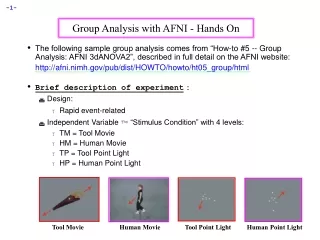
25. 3dANOVA3: A test case • Michael S. Beauchamp, Kathryn E. Lee, James V. Haxby, and Alex Martin, fMRI Responses to Video and Point-Light Displays of Moving Humans and Manipulable Objects, Journal of Cognitive Neuroscience, 15: 991-1001 (2003). • Purpose is to study the organization of brain responses to different types of complex visual motion (the 4 levels within factor A) from 9 subjects (the levels within factor B) • Data from 3 of the subjects, and scripts to process it with AFNI programs, are available in AFNI HowTo #5 (hands-on) • Available for download at the AFNI web site: http://afni.nimh.nih.gov/afni/doc/howto/ • If you want all the data, it is at the FMRI Data Center at Dartmouth: http://www.fmridc.org • Or at least, it should be (but they haven’t posted it yet for some reason)

26. Tool motion (TM) • Stimuli: Video clips of the following Human whole-body motion (HM) Human point motion (HP) Tool point motion (TP) From Figure 1 Beauchamp et al. 03 • Hypotheses to test: • Which areas are differentially activated by any of these stimuli (main effect)? • Which areas are differentially activated for point motion versus natural motion? (type of image) • Which areas are differentially activated for human-like versus tool-like motion? (type of motion)

27. Animations (file=beauchamp_videos.gif)

28. Data Processing Outline • Image registration with 3dvolreg • Images smoothed (4 mm FWHM) with 3dmerge • IRF for each of the 4 stimuli were obtained using 3dDeconvolve • Regressor coefficients (IRFs) were normalized to percent signal change (using 3dcalc) • An average activation measure was obtained by averaging IRF amplitude (using 3dTstat) • These activation measures will be the measurements in the ANOVA table • After each subject’s results are warped to Talairach coordinates, using adwarp program

29. Model type, number of levels for each factor Input for each cell in ANOVA table: totally 2X2X8 = 32 • Group Analysis: Example • Script 3dANOVA3 -type 4 -alevels 2 -blevels 2 -clevels 8 \ -dset 1 1 1 ED_TM_irf_mean+tlrc \ -dset 1 2 1 ED_TP_irf_mean+tlrc \ -dset 2 1 1 ED_HM_irf_mean+tlrc \ -dset 2 2 1 ED_HP_irf_mean+tlrc \ … -adiff 1 2 TvsH1 \ (indices for difference) -acontr 1 -1 TvsH2 \ (coefficients for contrast) -bdiff 1 2 MvsP1 \ -aBdiff 1 2 : 1 TMvsHM \ (indices for difference) -aBcontr 1 -1 : 1 TMvsHM \ (coefficients for contrast) -aBcontr -1 1 : 2 HPvsTP \ -Abdiff 1 : 1 2 TMvsTP \ -Abcontr 2 : 1 -1 HMvsHP \ -fa ObjEffect \ -fb AnimEffect \ -fab ObjXAnim \ -bucket Group 1st order Contrasts, paired t test 2nd order Contrasts, paired t test Main effects & interaction F test; Equivalent to contrasts Output: bundled

30. 4 & 5-Way ANOVA: ready to rock-n-roll (for the daring and intrepid) • Interactive Matlab script (user-friendly) • Can run both crossed and nested (i.e., subject nested into gender) design • Heavy duty computation + Matlab: expect to take 10s of minutes to hours • Same script can also do ANOVA, ANOVA2, and ANOVA3 analyses • Includes contrast tests across all factors • Balanced design with no missing data in most cases • Unbalanced design allowed with unequal number of subject across groups (e.g., unequal number of males and females). Much simpler than using 3dRegAna

31. 5 Types of 4-Way ANOVA

32. 3 Design Types of 5-Way ANOVA • A real example with 5-way mixed design (neural mechanism for category-selective response): • Factors • Task (between-subject): semantic decision, naming • Modality: visual, auditory • Format: verbal, nonverbal • Category: animal, tool • Subject (random) • 4 stimuli (2X2) for animal and tool - visual verbal = word, visual nonverbal = picture, auditory verbal = spoken, auditory nonverbal = sound • 4-way mixed design: Only 2 levels for all 3 within-subject factors: no concern for sphericity violation

33. Regression Analysis: 3dRegAna • Simple linear regression: • Y = b0 + b1X1,+ e • where Y represents the FMRI measurement (i.e., percent signal change) and X is the independent variable (i.e., drug dose) • Multiple linear regression: • Y = b0 + b1X1 + b2X2 + b3X3 + …+ e • Regression with qualitative and quantitative variables (ANCOVA) • i.e., drug dose (5mg, 12mg, 23mg, etc.) is quantitative while drug type (Nicotine, THC, Cocaine) or age group (young vs. old) or genotype is qualitative, and usually called dummy (or indicator) variable • ANOVA with unequal sample sizes (with indicator variables) • Polynomial regression: • Y = b0 + b1X1 + b2X12 + … + e • Linear regression: model is a linear function of its unknowns bi , NOT its independent variables Xi • Not for fitting time series, use 3dDeconvolve (or 3dNLfim) instead

34. F-test for Lack of Fit (lof) • If multiple measurements are available (and they should be), a Lack Of Fit (lof) test is first carried out. • Hypothesis: H0: E(Y) = b0 + b1X1 + b2X2 + …,+ bp-1Xp-1 Ha: E(Y) ≠b0 + b1X1 + b2X2 + …,+ bp-1Xp-1 • Hypothesis is tested by comparing the variance of the model’s lack of fit to the measurement variance at each point (pure error). • If Flof is significantthen model is inadequate. STOP HERE. • Reconsider independent variables, try again. • If Flof is insignificant then model appears adequate, so far. • It is important to test for the lack of fit: • The remainder of the analysis assumes an adequate model is used • You will not be visually inspecting the goodness of the fit for thousands of voxels!

35. Test for Significance of Linear Regression • This is done by testing whether additional parameters significantly improve the fit • For simple case Y=b0+b1X1 +e H0: b1=0 H1: b1≠ 0 • For general case Y = b0+b1X1 +b2X2 + … +bq-1Xq-1 +bqXq + … +bp-1Xp-1 +e H0: bq=bq+1=...=bp-1=0 Ha: bk≠ 0, for some k, q ≤ k ≤ p-1 • Freg is the F-statistic for determining if the Full model significantly improved on the reduced model • NOTE: This F-statistic is assumed to have a central F-distribution. This is not the case when there is a lack of fit

36. 3dRegAna: Other statistics • How well does model fit data? • R2 (coefficient of multiple determination) is the proportion of the variance in the data accounted for by the model 0 ≤ R2≤ 1. • i.e., if R2 = 0.26 then 26% of the data’s variation about their mean is accounted for by the model. So this might indicate the model, even if significant, might not be that useful (depends on what use you have in mind) • Having said that, you should consider R2 relative to the maximum it can achieve given the pure error which cannot be modeled. [cf. Draper & Smith, chapter 2]. • Are individual parameters bk significant? • t-statistic is calculated for each parameter • helps identify parameters that can be discarded to simplify the model • R2 and t-statistic are computed for full (not reduced) model

37. Examples from Applied Regression Analysis by Draper and Smith (third edition)

38. 3dRegAna: Qualitative Variables (ANCOVA) • See latest examples here: http://afni.nimh.nih.gov/sscc/gangc/ANCOVA.html • Qualitative variables can also be used • i.e., We’re modeling the response amplitude to a stimulus of varying contrast when subjects are either young, middle-aged or old. • X1 represents the stimulus contrast (quantitative): continuous covariate • Create indicator variables X2 and X3 to represent age: • X2 = 1 if subject is middle-aged = 0 otherwise • X3 = 1 if subject is old (i.e., at least 1 year older than Bob Cox) = 0 otherwise • Full Model (no interactions between age and contrast) • Y = b0+b1X1 +b2X2 +b3X3 +e • E(Y) = b0+b1X1 for young subjects • E(Y) = ( b0+b2 )+b1X1 for middle-aged subjects • E(Y) = ( b0+b3 )+b1X1 for old subjects • Full Model (with interactions between age and contrast) • Y = b0+b1X1 +b2X2 +b3X3 +b4X2X1 +b5X3X1 +e • E(Y) = b0+b1X1 for young subjects • E(Y) = ( b0+b2 )+ ( b1+b4 )X1 for middle-aged subjects • E(Y) = ( b0+b3 )+ ( b1+b5 )X1 for old subjects

39. Cluster Analysis: Multiple testing correction • Multiple testing problem in fMRI: voxel-wise statistical analysis • Increase of chance at least one detection is wrong in cluster analysis • Two approaches • Control FWE: aFW = P (≥ one false positive voxel in the whole brain) • Making aFW small but without losing too much power • Bonferroni correction doesn’t work: p=10-8~10-6 *Too stringent and overly conservative: Lose statistical power • Something to rescue? Correlation and structure! *Voxels in the brain are not independent *Structures in the brain • Control false discovery rate (FDR) • FDR = expected proportion of false + voxels among all detected voxels

40. Cluster Analysis: AlphaSim • FWE: Monte Carlo simulations • Named for Monte Carlo, Monaco, where the primary attractions are casinos • Program: AlphaSim • Randomly generate some number (e.g., 1000) of brains with false positive voxels • See what clusters form by chance alone, given spatial smoothness in data • Parameters: * ROI * Spatial correlation * Connectivity * Individual voxel significacet level (uncorrected p) • Output * Simulated (estimated) overall significance level (corrected p-value) * Corresponding minimum cluster size • Decision: Counterbalance among * Uncorrected p • * Minimum cluster size • * Corrected p

41. Program Restrict correcting region: ROI Spatial correlation Connectivity: how clusters are defined • Cluster Analysis: AlphaSim • Example AlphaSim \ -mask MyMask+orig \ -fwhmx 4.5 -fwhmy 4.5 -fwhmz 6.5 \ -rmm 6.3 \ -pthr 0.0001 \ -iter 1000 • FWHM are estimated using 3dFWHM: see http://afni.nimh.nih.gov/sscc/gangc/mcc.html • Output: 5 columns • Focus on the 1st and last columns, and ignore others • 1st column: minimum cluster size in voxels • Last column: alpha (a), overall significance level (corrected p value) Cl Size Frequency Cum Prop p/Voxel Max Freq Alpha2 1226 0.999152 0.00509459 831 0.859 3 25 0.998382 0.00015946 25 0.137 4 3 1.0 0.00002432 3 0.03 • May have to run several times with different uncorrected p: • increase uncorrected p --> increase in minimum cluster size Uncorrected p Number of simulations

42. Cluster Analysis: 3dFDR • Definition: FDR = proportion of false + voxels among all detected voxels • Doesn’t consider • spatial correlation • cluster size • connectivity • Again, only controls the expected % false positives among declared active voxels • Algorithm: statistic (t)  p value  FDR (q value)  z score • Example: 3dFDR -input ‘Group+tlrc[6]' \ -mask_file mask+tlrc \ -cdep -list \ -output test One statistic ROI Arbitrary distribution of p Output

43. Cluster Analysis: FWE or FDR? Correct type I error in different sense FWE: aFW = P (≥ one false positive voxel in the whole brain) Frequentist’s perspective: Probability among many hypothetical activation brains Used usually for parametric testing FDR = expected % false + voxels among all detected voxels Focus: controlling false + among detected voxels in one brain More frequently used in non-parametric testing Fail to survive correction? At the mercy of reviewers Analysis on surface Tricks One-tail? ROI – (the partial truth and nothing but the partial truth, so help you God)? Many factors along the pipeline Experiment design: power? Filtering FWHM and minimum cluster size Poor spatial alignment among subjects

44. Cluster Analysis: Conjunction analysis • Conjunction analysis • Common activation area • Exclusive activations • Double/dual thresholding with AFNI GUI • Tricky • Only works for two contrasts • Common but not exclusive areas • Conjunction analysis with 3dcalc • Flexible and versatile • Heaviside unit (step function) defines a On/Off event

45. Cluster Analysis: Conjunction analysis • Example with 3 contrasts: A vs D, B vs D, and C vs D • Map 3 contrasts to 3 numbers: A > D: 1; B > D: 2; C > D: 4 (why 4?) • Create a mask with 3 subbricks of t (all with a threshold of 4.2) 3dcalc -a func+tlrc'[5]' -b func+tlrc'[10]' -c func+tlrc'[15]‘ \ -expr 'step(a-4.2)+2*step(b-4.2)+4*step(c-4.2)' \ -prefix ConjAna • 8 (=23) scenarios: 0: none; 1: A > D but no others; 2: B > D but no others; 3: A > D and B > D but not C > D; 4: C > D but no others; 5: A > D and C > D but not B > D; 6: B > D and C > D but not A > D; 7: A > D, B > D and C > D

46. Need Help? Command with “-help” 3dANOVA3 -help Manuals http://afni.nimh.nih.gov/afni/doc/manual/ Web http://afni.nimh.nih.gov/sscc/gangc Examples: HowTo#5 http://afni.nimh.nih.gov/afni/doc/howto/ Message board http://afni.nimh.nih.gov/afni/community/board/ Appointment Contact us @1-800-NIH-AFNI