Hands-On Group Analysis with AFNI: 3-Way ANOVA Example
450 likes | 482 Vues
Learn to conduct a group analysis using AFNI's 3-Way ANOVA approach. This hands-on guide includes data processing steps and discussions on experiment data. Follow the provided script using afni_proc.py and explore the results.

Hands-On Group Analysis with AFNI: 3-Way ANOVA Example
E N D
Presentation Transcript
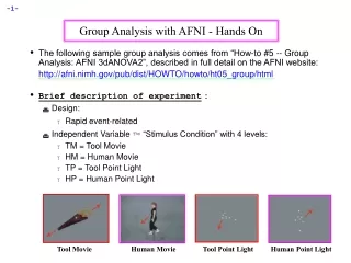
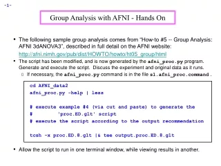
Group Analysis with AFNI - Hands On • The following sample group analysis comes from “How-to #5 -- Group Analysis: AFNI 3dANOVA3”, described in full detail on the AFNI website: http://afni.nimh.gov/pub/dist/HOWTO/howto/ht05_group/html • The script has been modified, and is now generated by the afni_proc.py program. Generate and execute the script. Discuss the experiment and original data as it runs. • If necessary, the afni_proc.py command is in the file s1.afni_proc.command . cd AFNI_data2 afni_proc.py -help | less # execute example #4 (via cut and paste) to generate the # 'proc.ED.glt' script # execute the script according to the output recommendation tcsh -x proc.ED.8.glt |& tee output.proc.ED.8.glt • Allow the script to run in one terminal window, while viewing results in another.
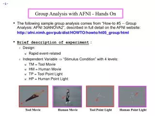
Brief description of experiment: • Design: Rapid event-related • stimulus or fixation presented randomly on a 1-second time grid • There are 4 stimulus types: Tool Point Light Human Point Light Tool Movie Human Movie • Data Collected: • 1 Anatomical (SPGR) dataset for each subject • 124 sagittal slices • 10 Time Series (EPI) datasets for each subject • 23 axial slices x 138 volumes = 3174 slices per run • TR = 2 sec; voxel dimensions = 3.75 x 3.75 x 5 mm • Sample size, n=7 (subjects ED, EE, EF, FH, FK, FL, FN)
Analysis Steps: • Part I: Process data for each subject • Pre-process subjects’ data many steps involved here… • Run deconvolution analysis on each subject’s dataset --- 3dDeconvolve • Part II: Run group analysis • warp results to standard space • 3-way Analysis of Variance (ANOVA) --- 3dANOVA3 • Object Type (2) x Animation Type (2) x Subjects (7) = 3-way ANOVA • Class work for Part I: • view the original data by running afni from the ED directory • then view output data from the ED.8.glt.results directory cd ED afni &
PART I Process Data for each Subject First: • Hands-on example: Subject ED • We will begin with ED’s anat dataset and 10 time-series (3D+time) datasets: EDspgr+orig, EDspgr+tlrc, ED_r01+orig, ED_r02+orig … ED_r10+orig • Below is ED’s ED_r01+orig (3D+time) dataset. Notice the first two time points of the time series have relatively high intensities*. We will need to remove them later: Timepoints 0 and 1 have high intensity values • Images obtained during the first 4-6 seconds of scanning will have much larger intensities than images in the rest of the timeseries, when magnetization (and therefore intensity) has decreased to its steady state value
Pre-processing is done by the proc.ED.8.glt script within the directory, AFNI_data2/ED.8.glt.results . • go to the ED.8.glt.results directory to start viewing the results • also, open the proc.ED.8.glt script in an editor (such as gedit), and follow the script while viewing the results • starting from the ED directory (from the previous slides)… cd .. gedit proc.ED.8.glt & cd ED.8.glt.results ls afni & • note that in the script, the count command is used to set the $runs variable as a list of run indices: • set runs = ( `count -digits 2 1 10` ) becomes: • set runs = ( 01 02 03 04 05 06 07 08 09 10 ) • And so: • foreach run ( $runs ) becomes: • foreach run ( 01 02 03 04 05 06 07 08 09 10 )
STEP 0 (tcat): Apply 3dTcat to copy datasets into the results directory, while removing the first 2 TRs from each run. • The first 2 TRs from each run occurred before the scanner reached a steady state. 3dTcat -prefix $output_dir/pb00.$subj.r01.tcat \ ED/ED_r01+orig'[2..$]' • The output datasets are placed into $output_dir, which is the results directory. • Using sub-brick selector '[2..$]' sub-bricks 0 and 1 will be skipped. • The '$' character denotes the last sub-brick. • The single quotes prevent the shell from interpreting the '[' and '$' characters. • The output dataset name format is: pb00.$subj.r01.tcat (.HEAD / .BRICK) • pb00 : process block 00 • $subj : the subject ID (ED.8.glt, in this case) • r01 : EPI data from run 1 • tcat : the name of this processing block (according to afni_proc.py) (other block names are tshift, volreg, blur, mask, scale, regress)
STEP 1 (tshift): Check for possible “outliers” in each of the 10 time series datasets using 3dToutcount . Then perform temporal alignment using 3dTshift. • An outlier is usually seen as an isolated spike in the data, which may be due to a number of factors, such as subject head motion or scanner irregularities. • The outlier is not a true signal that results from presentation of a stimulus event, but rather, an artifact from something else -- it is noise. foreach run (01 02 03 04 05 06 07 08 09 10) 3dToutcount -automask pb00.$subj.r$run.tcat+orig \ > outcount_r$run.1D end • How does this program work? For each time series, the trend and Mean AbsoluteDeviation are calculated. Points far away from the trend are considered outliers. • "far away" is defined as at least 5.43*MAD (for a time series of 136 TRs) • see 3dToutcount -help for specifics • -automask: do the outlier check only on voxels within the brain and ignore background voxels (which are detected by the program because of their smaller intensity values) • > : redirect output to the text file outcount_r01.1D (for example), instead of sending it to the terminal window.
Note: “1D” is used to identify a numerical text file. In this case, each file consists a column of 136 numbers (b/c of 136 time points). • Subject ED’s outlier files: outcount_r01.1D outcount_r02.1D … outcount_r10.1D • Use AFNI 1dplot to display any one of ED’s outlier files. For example: 1dplot outcount_r04.1D number of ‘outlier’ voxels, per TR Outliers? Inspect the data. High intensity values in the beginning are usually due to scanner attempting to reach steady state. time
in afni, view run 04, time points 117, 118 and 119 (0-based) • while it appears that something happened at time point 118 (such as a swallow, or similar movement), it may not be enough to worry about • if there had been a more significant problem, and if it could not be fixed by 3dvolreg, then it might be good to censor this time point via the -censor option in 3dDeconvolve internal movement can be seen in this area, using afni
Next, perform temporal alignment using 3dTshift. • Slices were acquired in an interleaved manner (slice 0, 2, 4, …, 1, 3, 5, …). • Interpolate each voxel's time series onto a new time grid, as if each entire volume had been acquired at the beginning of the TR. • For example, slice #0 was acquired at times t = 0, 2, 4, etc., in seconds. Slice #1 was acquired at times t = 1.043, 3.043, 5.043, etc. • After applying 3dTshift, all slices will have offset times of t = 0, 2, 4, etc. 3dTshift -tzero 0 -quintic \ -prefix pb01.$subj.r$run.tshift \ pb00.$subj.r$run.tcat+orig • -tzero 0 : the offset for each slice is set to the beginning of the TR • -quintic : interpolate using a 5th degree polynomial
Subject ED’s newly created time shifted datasets: pb01.ED.8.glt.r01.tshift+orig (.HEAD/.BRIK) ... pb01.ED.8.glt.r10.tshift+orig (.HEAD/.BRIK) • Below is run 01 of ED’s time shifted dataset. 4 2 Slice acquisition now in synchrony with beginning of TR 0
STEP 2: Register the volumes in each 3D+time dataset using AFNI program3dvolreg. Register all volumes to the third of the session. foreach run ( $runs ) 3dvolreg -verbose -zpad 1 \ -base pb01.$subj.r01.tshift+orig'[2]' \ -1Dfile dfile.r$run.1D \ -prefix pb02.$subj.r$run.volreg \ pb01.$subj.r$run.tshift+orig end cat dfile.r??.1D > dfile.rall.1D • -verbose: prints out progress report onto screen • -zpad : add one temporary zero slice on either end of volume • -base : align to third volume, since anatomy was scanned before EPI • -1Dfile : save motion parameters for each run (roll, pitch, yaw, dS, dL, dP) into a file containing 6 ASCII formatted columns • -prefix : output dataset names reflect processing block 2, volreg • input datasets are from processing block 1, tshift • concatenate the registration parameters from all 10 runs into one file
Subject ED’s 10 newly created volume registered datasets: pb02.ED.8.glt.r01.volreg+orig (.HEAD/.BRIK) ... pb02.ED.8.glt.r10.volreg+orig (.HEAD/.BRIK) • Below is run 01 of ED’s volume registered datasets.
view the registration parameters in the text file, dfile.rall.1D • this is the concatenation of the registration files for all 10 runs 1dplot -volreg dfile.rall.1D • very little movement is apparent - a good subject
STEP 3: Apply a Gaussian filter to spatially blur the volumes using program 3dmerge. • result is somewhat cleaner, more contiguous activation blobs • also helps account for subject variability when warping to standard space • spatial blurring will be done on ED’s time shifted, volume registered datasets foreach run ( $runs ) 3dmerge -1blur_fwhm 4 -doall \ -prefix pb03.$subj.r$run.blur \ pb02.$subj.r$run.volreg+orig end • -1blur_fwhm 4: use a full width half max of 4mm for the filter size • -doall : apply the editing option (in this case the Gaussian filter) to all sub-bricks in each dataset
results from 3dmerge: pb02.ED.8.glt.r01.volreg+orig pb03.ED.8.glt.r01.blur+orig Before blurring After blurring
STEP 3.5 (unnumbered block): creating a union mask • use 3dAutomask to create a 'brain' mask for each run • create a mask which is the union of the run masks • this mask can be applied in various ways: • during the scaling operation • in 3dDeconvolve (so that time is not wasted on background voxels) • to group data, in standard space • may want to use the intersection of all subject masks foreach run ( $runs ) 3dAutomask -dilate 1 -prefix rm.mask_r$run \ pb03.$subj.r$run.blur+orig end • -dilate 1 : dilate the mask by one voxel
next, take the union of the run masks • the mask datasets have values of 0 and 1 • can take union by computing the mean and comparing to 0.0 • other methods exist, but this is done in just two simple commands 3dMean -datum short -prefix rm.mean rm.mask*.HEAD 3dcalc -a rm.mean+orig -expr 'ispositive(a-0)' \ -prefix full_mask.$subj • -datum short : force full_mask to be of type short • rm.* files : these files will be removed later in the script • -a rm.mean+orig : specify the dataset used for any 'a' in '-expr' • -expr 'ispositive(a-0)': evaluates to 1 whenever 'a' is positive • note that the comparison to 0 can be changed • 0.99 would create an intersection mask • 0.49 would mean at least half of the masks are set
so the result is dataset, full_mask.ED.8.glt+orig • view this in afni • load pb03.ED.8.glt.r01.blur+orig as the underlay • load the mask dataset as the overlay • set the color overlay opacity to 5 • allows the underlay to show through the overlay color overlay opacity arrows
STEP 4: Scaling the Data - as percent of the mean • for each run • for each voxel • compute the mean value of the time series • scale the time series so that the new mean is 100 • scaling becomes an important issue when comparing data across subjects • using only one scanner, shimming affects the magnetization differently for each subject (and therefore affects the data differently for each subject) • different scanners might produce vastly different EPI signal values • without scaling, the magnitude of the beta weights may have meaning only when compared with other beta weights in the dataset • What does a beta weight of 4.7 mean? Basically nothing, by itself. • It is a small response, if many voxels have responses in the hundreds. • It is a large response, if it is a percentage of the mean. • by converting to percent change, we can compare the activation calibrated with the relative change of signal, instead of the arbitrary baseline of FMRI signal
For example: Subject 1 - signal in hippocampus has a mean of 1000, and goes from a baseline of 990 to a response at 1040 Difference = 50 MRI units Subject 2 - signal in hippocampus has a mean of 500, and goes from a baseline of 500 to a response at 525 Difference = 25 MRI units • Conclusion: each shows a 5% change, relative to the mean. • these changes are 5% above the baseline • But 5% of what? It is 5% of the mean. • Percent of baseline might be a slightly preferable scale (to percent of mean), but it may not be worth the price. • the difference is only a fraction of the result • e.g. a 5% change from the mean would be approximately a 5.1% change from the baseline, if the mean is 2% above the baseline • computing the baseline accurately is confounded by using motion parameters (but using motion parameters may be considered more important)
foreach run ( $runs ) 3dTstat -prefix rm.mean_r$run pb03.$subj.r$run.blur+orig 3dcalc -a pb03.$subj.r$run.blur_orig -b rm.mean_r$run+orig \ -c full_mask.$subj+orig \ -expr 'c * min(200, a/b*100)' \ -prefix pb04.$subj.r$run.scale end • dataset a : the blurred EPI time series (for a single run) • dataset b : a single sub-brick, where each voxel has the mean value for that run • dataset c : the full mask • -expr 'c * min(200, a/b*100)' • compute a/b*100 (the EPI value 'a', as a percent of the mean 'b') • if that value is greater than 200, use 200 • multiply by the mask value, which is 1 inside the mask, and 0 outside
compare EPI graphs from before and after scaling • they look identical, except for the scaling of the values • the EPI run 01 mean at this voxel is 1462.17 in the blur dataset (so dividing by 14.6217 gives the scaled values for this voxel) pb03.ED.glt.r01.blur+orig pb04.ED.glt.r01.scale+orig right-click in the center voxel of the graph window
compare EPI images from before and after scaling • the background voxels are all 0, because of applying the mask • the scaled image looks like a mask, because all values are either 0, or are close to 100 pb03.ED.glt.r01.blur+orig pb04.ED.glt.r01.scale+orig
STEP 5: Perform a deconvolution analysis on Subject ED’s data with 3dDeconvolve • What is the difference between regular linear regression and deconvolution? • With linear regression, the hemodynamic response is assumed. • With deconvolution, the hemodynamic response is not assumed. Instead, it is computed by3dDeconvolve from the data. • TENT(0,14,8) was chosen as the set of basis functions for each response • the response is to be computed from 0 seconds after each stimulus, to 14 seconds after each stimulus • 8 TENT functions will be used, over 7 two-second intervals • making each estimated response locked to the TR grid • TENT #0 and TENT #7, at the interval endpoints, are half TENTs
10 input datasets • 3dDeconvolve command - Part 1 3dDeconvolve -input pb04.$subj.r??.scale+orig.HEAD \ -polort 2 \ -mask full_mask.$subj+orig \ -basis_normall 1 \ -num_stimts 10 \ -stim_times 1 stimuli/stim_times.01.1D 'TENT(0,14,8)' \ -stim_label 1ToolMovie \ -stim_times 2 stimuli/stim_times.02.1D 'TENT(0,14,8)' \ -stim_label 2HumanMovie \ -stim_times 3 stimuli/stim_times.03.1D 'TENT(0,14,8)' \ -stim_label 3ToolPoint \ -stim_times 4 stimuli/stim_times.04.1D 'TENT(0,14,8)' \ -stim_label 4HumanPoint \ . . . continued on next page • see input dataset list by typing: echo pb04.$subj.r??.scale+orig.HEAD • use mask to avoid computation on zero-valued time series • use -basis_normall to specify that all basis functions have a height of 1 • first 4 (of 10) stimuli are given using -stim_times
3dDeconvolve command - Part 2 -stim_file 5 dfile.all.1D’[0]’-stim_base 5 \ -stim_file 6 dfile.all.1D’[1]’ -stim_base 6 \ -stim_file 7 dfile.all.1D’[2]’ -stim_base 7 \ -stim_file 8 dfile.all.1D’[3]’ -stim_base 8 \ -stim_file 9 dfile.all.1D’[4]’ -stim_base 9 \ -stim_file 10 dfile.all.1D’[5]’ -stim_base 10 \ -iresp 1 iresp_ToolMovie.$subj \ -iresp 2 iresp_HumanMovie.$subj \ -iresp 3 iresp_ToolPoint.$subj \ -iresp 4 iresp_HumanPoint.$subj \ . . . continued on next page • recall that dfile.all.1D contains 6 columns of registration parameters • roll, pitch, yaw, dS, dL, dP • excluding reminder labels, such as '-stim_label 5 roll' • applying '-stim_base' excludes them from the full F-stats, like the baseline • output an impulse response time series, from the 8 TENT functions • see the iresp files by typing the command: ls iresp*
3dDeconvolve command - Part 3 (end of command) -gltsym ../misc_files/glt1.txt -glt_label 1 FullF \ -gltsym ../misc_files/glt2.txt -glt_label 2 HvsT \ -gltsym ../misc_files/glt3.txt -glt_label 3 MvsP \ -gltsym ../misc_files/glt4.txt -glt_label 4 HMvsHP \ -gltsym ../misc_files/glt5.txt -glt_label 5 TMvsTP \ -gltsym ../misc_files/glt6.txt -glt_label 6 HPvsTP \ -gltsym ../misc_files/glt7.txt -glt_label 7 HMvsTM \ -fout -tout -x1D Xmat.x1D \ -fitts fitts.$subj \ -bucket stats.$subj • to view a symbolic general linear test (such as #4), try the command: • cat ../misc_files/glt4.txt • output F and t-stats for each test • output the X matrix in a 1D text file (with NIML header), Xmat.x1D • output the time series of the model fit in fitts.ED.8.glt+orig • output all beta weights, glts and statistics on them into on them into one bucket dataset, stats.ED.8.glt+orig
-iresp 1 iresp_ToolMove.ED.8.glt • -iresp 2 iresp_Human_Movie.ED.8.glt • -iresp 3 iresp_ToolPoint.ED.8.glt • -iresp 4 iresp_HumanPoint.ED.8.glt • these output files contain the estimated Impulse Response Function for each stimulus type • the percent signal change is shown at each time point • below is the estimated IRF for Subject ED’s “Human Movies” (HM) condition: UnderLay: iresp_Human_Movie OverLay: stats (Full F-stat) Voxel: Jump to (ijk) : 18 44 12
After running 3dDeconvolve, an 'all_runs' dataset is created by concatenating the 10 scaled EPI time series datasets, using program 3dTcat. 3dTcat -prefix all_runs.$subj pb04.$subj.r??.scale+orig.HEAD • we can use the Double Plot graph feature to plot the all_runs dataset, along with the fitts dataset, in the same graph window • this shows how well we have modeled the data, at a given voxel location • the fit time series is the sum of each regressor (X matrix column) times its corresponding beta weight • the fit time series is the same as the input time series, minus the error • note that different locations in the brain respond better to some stimulus classes than others, generally, so the fit time series may overlap better after one type of stimulus than after another • voxel 18, 44, 12 has the largest F-stat in the dataset
usually, plot the all_runs dataset along with the fitts dataset • however, 10 runs is too much, so plot run 01 with the fitts • set the Underlay topb04.ED.8.glt.run01.scale+orig • in an image window, 'Jump to (ijk)' -> 18 44 12 • open a Graph window with one graph (m), and autoscale (a) • in the Graph window, Opt -> Tran 1D -> Dataset #N • in the Dataset #N plugin, choose dataset fitts, and choose color dk-blue • in the Graph window, Opt -> Double Plot -> Overlay for a fast event related design, this is a nice fit
It is the iresp data that will be used in the group analysis. • Focusing on voxel 18, 44, 12 of dataset iresp_Human_Movie, we can see that the IRF is 8 TRs long (0-7), as specified by TENT(0,14,8). • To run ANOVA, only one data point can exist at each voxel. • so the percent signal change values for the 8 TRs will be averaged • In the voxel displayed below, the mean percent signal change =1.642% note the peak note the average
STEP 6: Compute a voxel-by-voxel mean percent signal change with 3dTstat. • The following 3dTstat commands will compute a voxel-by-voxel mean for each iresp dataset, of which we have four: ToolMovie, HumanMovie, ToolPoint, HumanPoint. • Note that this is not part of the proc.ED.8.glt script. 3dTstat -prefix ED_TM_irf_mean iresp_ToolMovie.ED.8.glt+orig 3dTstat -prefix ED_HM_irf_mean iresp_HumanMovie.ED.8.glt+orig 3dTstat -prefix ED_TP_irf_mean iresp_ToolPoint.ED.8.glt+orig 3dTstat -prefix ED_HP_irf_mean iresp_HumanPoint.ED.8.glt+orig
STEP 9: Warp the mean IRF datasets for each subject to Talairach space, by applying the transformation in the anatomical datasets with adwarp. • For statistical comparisons made across subjects, all datasets -- including functional overlays -- should be standardized (e.g., Talairach format) to control for variability in brain shape and size foreach cond (TM HM TP HP) adwarp -apar EDspgr+tlrc -dxyz 3 \ -dpar ED_{$cond}_irf_mean+orig \ end • The output of adwarp will be four Talairach transformed IRF datasets. ED_TM_irf_mean+tlrc ED_HM_irf_mean+tlrc ED_TP_irf_mean+tlrc ED_HP_irf_mean+tlrc • We are now done with Part 1, Process Individual Subjects’ Data, for Subject ED • go back and follow the same steps for remaining subjects • We can now move on to Part 2, RUN GROUP ANALYSIS (ANOVA)
PART 2 Run Group Analysis (ANOVA3): • In our sample experiment, we have 3 factors (or Independent Variables) for our analysis of variance: “Stimulus Condition” and “Subjects” • IV 1: OBJECT TYPE 2 levels • Tools (T) • Humans (H) • IV 2: ANIMATION TYPE 2 levels • Movies (M) • Point-light displays (P) • IV 3: SUBJECTS 7 levels (note: this is a small sample size!) • Subjects ED, EE, EF, FH, FK, FL, FN • The mean IRF datasets from each subject will be needed for the ANOVA. Example: ED_TM_irf_mean+tlrcEE_TM_irf_mean+tlrcEF_TM_irf_mean+tlrc ED_HM_irf_mean+tlrcEE_HM_irf_mean+tlrcEF_HM_irf_mean+tlrc ED_TP_irf_mean+tlrcEE_TP_irf_mean+tlrcEF_TP_irf_mean+tlrc ED_HP_irf_mean+tlrcEE_HP_irf_mean+tlrcEF_HP_irf_mean+tlrc
IV’s A & B are fixed, C is random. See 3dANOVA3 -help • 3dANOVA3 Command - Part 1 3dANOVA3 -type 4 \ -alevels 2 \ -blevels 2 \ -clevels 7 \ -dset 1 1 1 ED_TM_irf_mean+tlrc \ -dset 2 1 1 ED_HM_irf_mean+tlrc \ -dset 1 2 1 ED_TP_irf_mean+tlrc \ -dset 2 2 1 ED_HP_irf_mean+tlrc \ -dset 1 1 2 EE_TM_irf_mean+tlrc \ -dset 2 1 2 EE_HM_irf_mean+tlrc \ -dset 1 2 2 EE_TP_irf_mean+tlrc \ -dset 2 2 2 EE_HP_irf_mean+tlrc \ -dset 1 1 3 EF_TM_irf_mean+tlrc \ -dset 2 1 3 EF_HM_irf_mean+tlrc \ -dset 1 2 3 EF_TP_irf_mean+tlrc \ -dset 2 2 3 EF_HP_irf_mean+tlrc \ IV A: Object IV B: Animation IV C: Subjects irf datasets, created for each subj with 3dDeconvolve (See p.26) Continued on next page…
3dANOVA3 Command - Part 2 -dset 1 1 4 FH_TM_irf_mean+tlrc \ -dset 2 1 4 FH_HM_irf_mean+tlrc \ -dset 1 2 4 FH_TP_irf_mean+tlrc \ -dset 2 2 4 FH_HP_irf_mean+tlrc \ -dset 1 1 5 FK_TM_irf_mean+tlrc \ -dset 2 1 5 FK_HM_irf_mean+tlrc \ -dset 1 2 5 FK_TP_irf_mean+tlrc \ -dset 2 2 5 FK_HP_irf_mean+tlrc \ -dset 1 1 6 FL_TM_irf_mean+tlrc \ -dset 2 1 6 FL_HM_irf_mean+tlrc \ -dset 1 2 6 FL_TP_irf_mean+tlrc \ -dset 2 2 6 FL_HP_irf_mean+tlrc \ -dset 1 1 7 FN_TM_irf_mean+tlrc \ -dset 2 1 7 FN_HM_irf_mean+tlrc \ -dset 1 2 7 FN_TP_irf_mean+tlrc \ -dset 2 2 7 FN_HP_irf_mean+tlrc \ more irf datasets Continued on next page…
Produces main effect for factor ‘a’ (Object type), i.e., which voxels show increases in % signal change that is significantly different from zero? • 3dANOVA3 Command - Part 3 -fa ObjEffect \ -fb AnimEffect \ -adiff 1 2 TvsH \ -bdiff 1 2 MvsP \ -acontr 1 -1 sameas.TvsH \ -bcontr 1 -1 sameas.MvsP \ -aBcontr 1 -1: 1 TMvsHM \ -aBcontr -1 1: 2 HPvsTP \ -Abcontr 1: 1 -1 TMvsTP \ -Abcontr 2: 1 -1 HMvsHP \ -bucket AvgAnova Main effect for factor ‘b’, (Animation type) These are contrasts (t-tests). Explained on pp 38-39 All F-tests, t-tests, etc will go into this dataset bucket End of ANOVA command
-adiff: Performs contrasts between levels of factor ‘a’ (or -bdiff for factor ‘b’, -cdiff for factor ‘c’, etc), with no collapsing across levels of factor ‘a’. E.g.1, Factor “Object Type” --> 2 levels: (1)Tools, (2)Humans: -adiff 1 2 TvsH E.g., 2, Factor “Faces” --> 3 levels: (1)Happy, (2)Sad, (3)Neutral -adiff 1 2 HvsS -adiff 2 3 SvsN -adiff 1 3 HvsN • -acontr: Estimates contrasts among levels of factor ‘a’ (or -bcontr for factor ‘b’, -ccontr for factor ‘c’, etc). Allows for collapsing across levels of factor ‘a’ • In our example, since we only have 2 levels for both factors ‘a’ and ‘b’, the -diff and -contr options can be used interchangeably. Their different usages can only be demonstrated with a factor that has 3 or more levels: • E.g.: factor ‘a’ = FACES --> 3 levels :(1) Happy, (2) Sad, (3) Neutral -acontr -1 .5 .5 HvsSN -acontr .5 .5 -1 HSvsN -acontr .5 -1 .5 HNvsS Simple paired t-tests, no collapsing across levels, like Happy vs. Sad/Neutral Happy vs. Sad/Neutral Happy/Sad vs. Neutral Happy/Neutral vs. Sad
-aBcontr: 2nd order contrast. Performs comparison between 2 levels of factor ‘a’ at a Fixed level of factor ‘B’ • E.g. factor ‘a’ --> Tools(1) vs. Humans(-1), factor ‘B’ --> Movies(1) vs. Points(2) • We want to compare ‘Tools Movies’ vs. ‘Human Movies’. Ignore ‘Points’ -aBcontr 1 -1 : 1 TMvsHM • We want to compare “Tool Points’ vs. ‘Human Points’. Ignore ‘Movies’ -aBcontr 1 -1 : 2 TPvsHP • -Abcontr: 2nd order contrast. Performs comparison between 2 levels of factor ‘b’ at a Fixed level of factor ‘A’ • E.g., E.g. factor ‘b’ --> Movies(1) vs. Points(-1), factor ‘A’ --> Tools(1) vs. Humans(2) • We want to compare ‘Tools Movies’ vs. ‘Tool Points’. Ignore ‘Humans -Abcontr 1 : 1 -1 TMvsTP • We want to compare “Human Movies vs. ‘Human Points’. Ignore ‘Tools’ -Abcontr 2 : 1 -1 HMvsHP
In class -- Let’s run the ANOVA together: • cd AFNI_data2 • This directory contains a script called s3.anova.ht05 that will run 3dANOVA3 • This script can be viewed with a text editor, like emacs • ./s3.anova.ht05 • execute the ANOVA script from the command line • cd group_data ; ls • result from ANOVA script is a bucket dataset AvgANOVA+tlrc, stored in the group_data/ directory • afni & • launch AFNI to view the results • The output from 3dANOVA3 is bucket dataset AvgANOVA+tlrc, which contains 20 sub-bricks of data: • i.e., main effect F-tests for factors A and B, 1st order contrasts, and 2nd order contrasts
-fa: Produces a main effect for factor ‘a’ • In this example, -fa determines which voxels show a percent signal change that is significantly different from zero when any level of factor “Object Type” is presented • -fa ObjEffect: ULay: sample_anat+tlrc OLay: AvgANOVA+tlrc Activated areas respond to OBJECTS in general (i.e., humans and/or tools)
Brain areas corresponding to “Tools” (reds) vs. “Humans” (blues) • -diff 1 2 TvsH (or -acontr 1 -1 TvsH) ULay: sample_anat+tlrc OLay: AvgANOVA+tlrc Red blobs show statistically significant percent signal changes in response to “Tools.” Blue blobs show significant percent signal changes in response to “Humans” displays
Brain areas corresponding to “Human Movies” (reds) vs. “Humans Points” (blues) • -Abcontr 2: 1 -1 HMvsHP ULay: sample_anat+tlrc OLay: AvgANOVA+tlrc Red blobs show statistically significant percent signal changes in response to “Human Movies.” Blue blobs show significant percent signal changes in response to “Human Points” displays
Many thanks to Mike Beauchamp for donating the data used in this lecture and in the how-to#5 • For a full review of the experiment described in this lecture, see Beauchamp, M.S., Lee, K.E., Haxby, J.V., & Martin, A. (2003). FMRI responses to video and point-light displays of moving humans and manipulable objects. Journal of Cognitive Neuroscience, 15:7, 991-1001. • For more information on AFNI ANOVA programs, visit the web page of Gang Chen, our wise and infinitely patient statistician: http//afni.nimh.gov/sscc/gangc