Exploring the Binomial Test and Hypothesis Testing in ESP Claims
This text delves into the concept of hypothesis testing, particularly through the lens of the Binomial Test. Using an example where a friend claims to predict outcomes more accurately than chance, it outlines the process of formulating null and alternative hypotheses. The focus remains on determining whether claims of ESP (extrasensory perception) hold up under statistical scrutiny. The document explains concepts such as likelihood, critical values, and the errors associated with hypothesis testing. It also provides insights into treatment evaluation and the importance of understanding Type I and Type II errors.

Exploring the Binomial Test and Hypothesis Testing in ESP Claims
E N D
Presentation Transcript
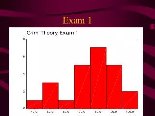
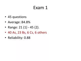
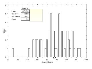
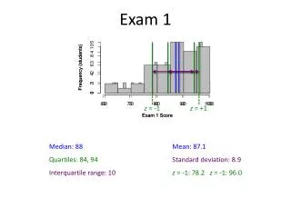
Exam 1 z = -1 z = +1 Median: 88 Quartiles: 84, 94 Interquartile range: 10 Mean: 87.1 Standard deviation: 8.9 z = -1: 78.2 z = -1: 96.0
ESP • Your friend claims he can predict the future • You flip a coin 5 times, and he’s right on 4 • Is your friend psychic?
Two Hypotheses • Hypothesis • A theory about how the world works • Proposed as an explanation for data • Posed as statement about population parameters • Psychic • Some ability to predict future • Not perfect, but better than chance • Luck • Random chance • Right half the time, wrong half the time • Hypothesis testing • A method that uses inferential statistics to decide which of two hypotheses the data support
Inference Population Sample Probability Support Hypotheses Statistics Likelihood Likelihood • Likelihood • Probability distribution of a statistic, according to each hypothesis • If result is likely according to a hypothesis, we say data “support” or “are consistent with” the hypothesis • Likelihood for f(correct) • Psychic: hard to say; how psychic? • Luck: can work out exactly; 50/50 chance each time
Binomial Distribution • Binary data • A set of two-choice outcomes, e.g. yes/no, right/wrong • Binomial variable • A statistic for binary samples • Frequency of “yes” / “right” / etc. • Binomial distribution • Probability distribution for a binomial variable • Gives probability for each possible value, from 0 to n • A family of distributions • Like Normal (need to specify mean and SD) • n: number of observations (sample size) • q: probability correct each time
n = 20, q = .5 n = 5, q = .5 n = 20, q = .25 n = 20, q = .5 Binomial Distribution Formula (optional): Frequency Frequency
Binomial Test • Hypothesis testing for binomial statistics • Null hypothesis • Some fixed value for q, usually q = .5 • Nothing interesting going on; blind chance (no ESP) • Alternative hypothesis • q equals something else • One outcome more likely than expected by chance (ESP) • Goal: Decide which hypothesis the data support • Strategy • Find likelihood distribution for f(Y) according to null hypothesis • Compare actual result to this distribution • If actual result is too extreme, reject null hypothesis and accept altenative hypothesis • “Innocent until proven guilty” • Believe null hypothesis unless compelling evidence to rule it out • Only accept ESP if luck can’t explain the data
Likelihood according to Luck: Binomial(n = 20, q = .5) Testing for ESP • Null hypothesis: Luck, q = .5 • Alternative hypothesis: ESP, q > .5 • Need to decide rules in advance • If too extreme, abandon luck and accept ESP • How unlikely before we will give up on Luck? • Where to draw cutoff? • Critical value: value our statistic must exceed to reject null hypothesis (Luck) Not at all unexpected Luck still a viable explanation Nearly impossible by luck alone Frequency
Another Example: Treatment Evaluation • Do people tend to get better with some treatment? • Less depression, higher WBC, better memory, etc. • Measure who improves and who worsens • Want more people better off than worse • Sign test • Ignore magnitude of change; just direction • Same logic as other binomial tests • Count number of patients improved • Compare to probabilities according to chance
Structure of a Binomial Test • Binary data • Each patient is Better or WorseEach coin prediction is Correct or Incorrect • Population parameter q • Probability each patient will improveProbability each guess will be correct • Null hypothesis, usually q = .5 • No effect of treatmentNo ESP • Better or worse equally likelyCorrect and incorrect equally likely • Alternative hypothesis, here q > .5 • Effective treatment; more people improveESP; guess right more often than chance • Work out likelihood according to null hypothesis • Probability distribution for f(improve)Probability distribution for f(correct) • Compare actual result to these probabilities • If more improve than likely by chance, If more correct than likely by chance, accept treatment is useful abandon luck and accept ESP • Need to decide critical value • How many patients must improve?How many times correct? Probability Frequency
Errors • Whatever the critical value, there will be errors • All values 0 to n are possible under null hypothesis • Even 20/20 happens once in 1,048,576 times • Can only minimize how often errors occur • Two kinds of errors: • Type I error • Null hypothesis is true, but we reject it • Conclude a useless treatment is effective • Type II error • Null hypothesis is false, but we don’t reject it • Don’t recognize when a treatment is effective
Critical Value and Error Rates Null Hypothesis (Bogus Treatments) Type I Errors Alternative Hypothesis(Effective Treatments) ? ? ? ? Type II Errors ? Frequency Frequency ? ? ? ? ? ? ? ?
Critical Value and Error Rates Null Hypothesis (Bogus Treatments) • Increasing critical value reduces Type I error rate but increases Type II error rate (and vice versa) • So, how do we decide critical value? • Two principles • Type I errors are more important to avoid • Can’t figure out Type II error rate anyway • Strategy • Decide how many Type I errors are acceptable • Choose critical value accordingly Type I Errors Alternative Hypothesis (Effective Treatments) ? ? ? ? Type II Errors ? Frequency Frequency ? ? ? ? ? ? ? ?
Controlling Type I Error Null Hypothesis (Bogus Treatments) • Type I error rate • Proportion of times, when null hypothesis is true, that we mistakenly reject it • Fraction of bogus treatments that we conclude are effective • Type I error rate equals total probability beyond the critical value, according to null hypothesis • Strategy • Decide what Type I error rate we want to allow • Pick critical value accordingly • Alpha level (a) • Chosen Type I error rate • Usually .05 in Psychology • Determines critical value Type I Error Rate Frequency
Summary of Hypothesis Testing Null Hypothesis (Bogus Treatments) • Determine Null and Alternative Hypotheses • Competing possibilities about a population parameter • Null is always precise; usually means “no effect” • Find probability distribution of test statistic according to null hypothesis • Likelihood of the statistic under that hypothesis • Choose acceptable rate of Type I errors (a) • Pick critical value of test statistic based on a • Under Null, probability of a result past critical value equals a • Compare actual result to critical value • If more extreme, reject Null as unable to explain data • Otherwise, stick with Null because it’s an adequate explanation Reject Null Keep Null Type I ErrorRate (a) Frequency
Review To test whether infants can read, you show pairs of good and bad words, and count how many times the baby crawls to the good word. What’s the null hypothesis? • Baby is more likely to crawl to good word • Baby is more likely to crawl to bad word • Baby is equally likely to crawl to either word • Baby will not choose either word Teddy bear Monster
Review What would be a Type II Error for this experiment? • Concluding babies can’t read when they really can • Concluding babies can read when they really can’t • Correctly concluding babies can read • Correctly concluding babies can’t read Teddy bear Monster
Review Each baby gets 6 trials. If any baby chooses the good word ≥5 times, you declare (s)he can read. Here are the probabilities of what will happen, according to the null hypothesis: What’s the Type I error rate? Number of good words 0 1 2 3 4 5 6 Probability .02 .09 .23 .31 .23 .09 .02 Correct answer is .11