Reasoning with Classical Propositional Logic
Reasoning with Classical Propositional Logic. Jacques Robin. Outline. Syntax Full CPL Implicative Normal Form CPL (INFCPL) Horn CPL (HCPL) Semantics Cognitive and Herbrand interpretations, models Reasoning FCPL Reasoning Truth-tabel based model checking Multiple inference rules

Reasoning with Classical Propositional Logic
E N D
Presentation Transcript
Reasoning with Classical Propositional Logic Jacques Robin
Outline • Syntax • Full CPL • Implicative Normal Form CPL (INFCPL) • Horn CPL (HCPL) • Semantics • Cognitive and Herbrand interpretations, models • Reasoning • FCPL Reasoning • Truth-tabel based model checking • Multiple inference rules • INFCPL Reasoning • Resolution and factoring • DPLL • WalkSat • HCPL Reasoning • Forward chaining • Backward chaining
FCPLUnaryConnective FCPLBinaryConnective Connective: enum{} Connective: enum{, , , } Arg Functor FCPLConnective ConstantSymbol 1..2 Full Classical Propositional Logic (FCPL): syntax Syntax (a (b ((c d) a) b)) FCPLFormula
INFCPLFormula CNFCPLFormula Functor = Functor = INFCPLClause CNFCPLClause NegativeLiteral INFCLPLHS INFCLPRHS Functor = Functor = Functor = Functor = Functor = CPL Normal Forms Implicative Normal Form (INF) Premisse * * * ConstantSymbol Conclusion • Semantic equivalence: • a b c d • (a b) c d • a b c d Conjunctive Normal Form (CNF) * * Literal ConstantSymbol
INFCPLFormula CNFCPLFormula Functor = Functor = CNFCPLClause INFCPLClause INFCLPLHS NegativeLiteral INFCLPRHS Functor = Functor = Functor = Functor = Functor = Horn CLP Implicative Normal Form (INF) Premisse * ConstantSymbol * Conclusion IntegrityConstraint a b c false context IntegrityConstraint inv IC: Conclusion.ConstantSymbol = false a b c d DefiniteClause context DefiniteClause inv DC: Conclusion.ConstantSymbol false Fact context Fact inv Fact: Premisse -> size() = 1 and Premisse -> ConstantSymbol = true true d Conjunctive Normal Form (CNF) * * Literal ConstantSymbol a b c IntegrityConstraint context IntegrityConstraint inv IC: Literal->forAll(oclIsKindOf(NegativeLiteral)) a b c d context DefiniteClause inv DC: Literal.oclIsKindOf(ConstantSymbol)->size() = 1 DefiniteClause context Fact inv Fact: Literal->forAll(oclIsKindOf(ConstantSymbol)) d Fact
FCPLUnaryConnective TruthValue FCPLBinaryConnective Connective: enum{} Value: enum{true,false} Connective: enum{, , , } FormulaMapping ConstantMapping CompoundDomainProperty AtomicDomainProperty FCPL semantics: cognitive interpretation Syntax (a (b ((c d) a) b)) Arg Functor FCPLConnective FCPLFormula ConstantSymbol 1..2 • fm1(pitIn12 pitIn11) = agent knows there is a pit in coordinates (1,2) and no pit in coordinates (1,1) fm1(pitIn12 pitIn11) = John is the Kind of England and John is not the King of France • csm1(pitIn12) = agent knows there is a pit in coordinates (1,2) • csm2(pitIn12) = John is the King of England FCLPCognitiveInterpretation Semantics
FCPLUnaryConnective TruthValue FCPLBinaryConnective Value: enum{true,false} Connective: enum{} Connective: enum{, , , } FormulaValuation ConstantValuation FCLPHerbrandModel FCPL semantics: Herbrand interpretation Syntax (a (b ((c d) a) b)) • {cv1(pitIn12) = true, cv1(pitIn11) = true, ...} • {cv2(pitIn12) = true, cv2(pitIn11) = false, ...} Arg Functor FCPLConnective FCPLFormula ConstantSymbol 1..2 FCLPHerbrandInterpretation • {fv1(pitIn12 pitIn11) = true, fv1(pitIn12 pitIn11) = true, ...} • {fv2(pitIn12 pitIn11) = true, fv2(pitIn12 pitIn11) = false, ...} Semantics
TruthValue FCPLUnaryConnective FCPLBinaryConnective Value: enum{true,false} Connective: enum{} Connective: enum{, , , } FCPL semantics Syntax (a (b ((c d) a) b)) Arg Functor FCPLConnective FCPLFormula ConstantSymbol 1..2 FormulaValuation ConstantValuation FormulaMapping FCLPHerbrandInterpretation FCLPCognitiveInterpretation ConstantMapping FCLPHerbrandModel CompoundDomainProperty AtomicDomainProperty Semantics
Valid formulas Satisfiable formulas Unsatisfiable formulas Entailment and models • Entailment |=: • f |= f’ iff: Hi, Hi(f) = true Hi(f’) = true • Logical equivalence : • f f’ iff f |= f’ and f’ |= f • Herbrand model: • An Herbrand interpretation Hi is a (Herbrand) model of formula f iffits truth value corresponds to the application of the truth-table definition of the FCPL connectives to the truth value in Hi of the constant symbols that compose f • f valid (or tautology) iff true in all Hi(f), ex, a a • f satisfiable iff true in at least one Hi(f) • f unsatisfiable (or contradiction) iff false in all Hi(f), ex, a a
Logic-Based Agent Given B as axiom, formula f is a theorem of L? B |=L f ? B f is valid in L? (Boolean CSP search proof) B f is unsatisfiable in L? (Refutation proof) • Strenghts: • Reuse results and insights about correct reasoning that matured over 23 centuries • Semantics (meaning) of a knowledge base can be represented formally as syntax, a key step towards automating reasoning Environment Sensors Ask Inference Engine: Theorem Prover for Logic L Knowledge Base B:Domain Model in Logic L Tell Retract Actuators
To answer: Ask() Enumerate all His from domain proposition alphabet Use truth-table to compute Mh(KB) and Mh() If Mh(KB) Mh(), then answer yes, else answer no Example: KB = pit11 breeze11 pit12 breeze12 1 = pit21 2 = pit22 Truth-table based model checking
Bi-directional (logical equivalences) R1: f g g f R2: f g g f R3: (f g) h f (g h) R4: (f g) h f (g h) R5: f f R6: f g g f R7: f g f g R8: f g (f g) (g f) R9: (f g) f g R10: (f g) f g R11: f (g h) (f g) (f h) R12: f (g h) (f g) (f h) R13: f f f %factoring Directed (logical entailments) R14: f g, f |= g %modus ponens R15: f g, g |= f %modus tollens R16: f g |= f %and-elimination R17: l1 ... li ... lk, m1 ... mj-1 li mj-1... mk|= l1 ... li-1 li-1... lk m1 ... mj-1 mj-1... mk %resolution FCLP inference rules
Idea: KB |= f ? KB0 = KB Apply inference rule: KBi |= g Update KBi+1 = KBi g Iterate until f KBkor until f KBn and KBn+1 = KBn Transforms proving KB |= f into search problem At each step: Which inference rule to apply? To which sub-formula of f? Example proof: KB0 = P1,1 (B1,1 P1,2 P2,1) (B2,1 P1,1 P2,2 P3,1) B1,1 B2,1 Query: (P1,2 P2,1) Cognitive interpretation: BX,Y: agent felt breeze in coordinate (X,Y) PX,Y: agent knows there is a pit in coordinate (X,Y) Apply R8 to B1,1 P1,2 P2,1KB1 = KB0 (B1,1 (P1,2 P2,1)) ((P1,2 P2,1) B1,1) Apply R6 to last sub-formula KB2 = KB1 (B1,1 (P1,2 P2,1)) Apply R14 to B1,1 andlast sub-formula KB3 = KB2 (P1,2 P2,1) Multiple inference rule application
Resolution and factoring • Repeated application of only two inference rules: • resolution and factoring • More efficient than using multiple inference rules • search space with far smaller branching factor • Refutation proof: • Derive false from KB Query • Requires both in normal form (conjunctive or implicative) • Example proof in conjunctive normal form:
Resolution strategies • Search heuristics for resolution-based theorem proving • Two heuristic classes: • Choice of clause pair to resolve inside current KB • Choice of literals to resolve inside chosen clause pair • Unit preference: • Prefer pairs with one unit clause (i.e., literals) • Rationale: generates smaller clauses, eliminates much literal choice in pair • Unit resolution: turn preference into requirement • Set of support: • Define small subset of initial clauses as initial “set of support” • At each step: • Only consider clause pairs with one member from current set of support • Add step result to set of support • Efficiency depend on cleverness of initial set of support • Common domain-independent initial set of support: negated query • Beyond efficiency, results in easier to understand, goal-directed proofs • Linear resolution: • At each step only consider pairs (f,g) where f is either: • (a) in KB0, or • (b) an ancestor of g in the proof tree • Input resolution: • Specialization of linear resolution excluding (b) case • Generates spine-looking proofs trees
FCPL theorem proving as boolean CSP exhaustive global backtracking search • Put f = KB Query in conjunctive normal form • Try to prove it unsatisfiable • Consider each literal in f as a boolean variable • Consider each clause in f as a constraint on these variables • Solve the underlying boolean CSP problem by using: • Exhaustive global backtracking search • of all complete variable assignments • showing nonesatisfies all constraint in f • Initial state: empty assignment of pre-ordered variables • Search operator: • Tentative assignment of next yet unassigned variable Li (ith literal in f) • Apply truth table definitions to propagate constraints in which Li appears (clauses of f involving L) • If propagation violates one constraint, backtrack on Li • If propagation satisfies all constraints: • iterate on Li+1 • if Li was last literal in f, fail, KB Query satisfiable, and thus KB | Query
V = [0,?,?] C = [1,?,?,?,?] V = [1,?,?] C = [0,?,?,?,?] V = [0,1,?] C = [1,0,?,?,1] V = [1,0,?] C = [0,1,?,?,0] V = [0,0,?] C = [1,0,?,?,0] V = [1,1,?] C = [0,0,?,?,1] V = [0,0,0] C = [1,0,0,0,0] V = [0,0,1] C = [1,0,0,0,0] V = [0,1,0] C = [1,0,0,0,1] V = [0,1,1] C = [1,0,0,1,1] V = [1,0,0] C = [0,1,1,0,0] V = [1,0,1] C = [0,1,0,0,0] V = [1,1,0] C = [0,0,1,0,1] V = [1,1,1] C = [0,0,0,0,1] FCPL theorem proving as boolean CSP backtracking search: example • Variables = {B1,1 , P1,2, P2,1} • Constraints: {B1,1 , P1,2 B1,1 , P2,1 B1,1, B1,1 P1,2 P2,1 , P1,2} V = [?,?,?] C = [?,?,?,?,?]
DPLL algorithm • General purpose CSP backtracking search very inefficient for proving large CFPL theorems • Davis, Putnam, Logemann & Loveland algorithm (DPPL): • Specialization of CSP backtracking search • Exploiting specificity of CFPL theorem proving recast as CSP search • To apply search completeness preserving heuristics • Concepts: • Pure symbol S: yet unassigned variable positive in all clauses or negated in all clauses • Unit clause C: clause with all but one literal already assigned to false • Heuristics: • Pure symbol heuristic: assign pure symbols first • Unit propagation: • Assign unit clause literals first • Recursively generate new ones • Early termination heuristic: • After assigning Li = true, propagate Cj = trueCj | Li Cj (avoiding truth-table look-ups) • Prune sub-tree below any node where Cj | Cj = false • Clause learning
Satisfiability of formula as boolean CSP heuristic local stochastic search • DPLL is not restricted to proving entailment by proving unsatisfiability • It can also prove satisfiability of a FCPL formula • Many problems in computer science and AI can be recast as a satisfiability problem • Heuristic local stochastic boolean CSP search more space scalable than DPLL for satisfiability • However since it is notexhaustive search, it cannotprove unsatisfiability (and thus entailment), only strongly suspect it • WalkSAT • Initial state: random assignment of pre-ordered variables • Search operator: • Pick a yet unsatisfied clause and one literal in it • Flip the literal assignment • At each step, randomly chose between to picking strategies: • Pick literal which flip results in steepest decrease in number of yet unsatisfied clauses • Random pick
Domain Specific • Agent Decision Problem • Search Model: • State data structure • Successor function • Goal function • Heuristic function Domain Independent Search Algorithm Reasoning Component Developer Agent Decision Problem Agent Application Developer • Domain Independent Inference Engine Search Model • State data structure • Successor function • Goal function • Heuristic function • Domain Specific • Knowledge Base Model: • Logic formulas true d f g h c ... Direct x indirect use of search for agent reasoning
Horn CPL reasoning • Practical limitations of FCPL reasoning: • For experts in most application domain (medicine, law, business, design, troubleshooting): • Non-intuitiveness of FCPL formulas for knowledge acquisition • Non-intuitiveness of proofs generated by FCPL algorithms for knowledge validation • Theoretical limitation of FCPL reasoning: • exponential in the size of the KB • Syntactic limitation to Horn clauses overcome both limitations: • KB becomes base of simple rules If p1 and ... and pn then c, with logical semantics p1 ... pn c • Two algorithms are available, rule forward chaining and rule backward chaining, that are: • Intuitive • Sound and complete for HCPL • Linear in the size of the KB • For most application domains, loss of expressiveness can be overcome by addition of new symbols and clauses: • ex, FCPL KB1 = p q c d has no logical equivalent in HCPL in terms of alphabet {p,q,c,d} • However KB2 = (p q notd c) (p q notc d) (c notc false) (d notd false) is an HCPL formula logically equivalent to KB1
Propositional forward chaining • Repeated application of modus ponens until reaching a fixed point • At each step i: • Fire all rules (i.e., Horn clauses with at least one positive and one negative literal) with all premises already in KBi • Add their respective conclusions to KBi+1 • Fixed point k reached when KBk =KBk-1 • KBk = {f | KB0 |= f}, i.e.,all logical conclusions of KB0 • If f KBk, then KB0 |= f, otherwise, KB0 | f • Naturally data-driven reasoning: • Guided by fact (axioms) in KB0 • Allows intuitive, direct implementation of reactive agents • Generally inefficient for: • Inefficient for specific entailment query • Cumbersome for deliberative agent implementations • Builds and-or proof graph bottom-up
Propositional backward chaining • Repeated application of resolution using: • Unit input resolution strategy with negated query as initial set of support • At each step i: • Search KB0 for clause of the form p1... pn g to resolve with clause g popped from the goal stack • If there are several ones, pick one, push p1... pn on goal stack, and push other ones alternative stack to consider upon backtracking • If there are none, backtrack (i.e., pop alternative stack) • Terminates: • Successfully when goal stack is empty • As failure when goal stack is non empty but alternative stack is • Naturally goal-driven reasoning: • Guided by goal (theorem to prove) • Allows intuitive, direct implementation of deliberative agents • Generally: • Inefficient for deriving all logical conclusions from KB • Cumbersome implementation of reactive agents • Builds and-or proof graph top-down
Propositional backward chaining: example Goal Stack Q Alternative Stack
Propositional backward chaining: example Goal Stack P Alternative Stack
Propositional backward chaining: example Goal Stack L M Alternative Stack
Propositional backward chaining: example Goal Stack A P M Alternative Stack A B
Propositional backward chaining: example Goal Stack P M Alternative Stack A B
Propositional backward chaining: example Goal Stack A B M Alternative Stack
Propositional backward chaining: example Goal Stack M Alternative Stack
Propositional backward chaining: example Goal Stack B L Alternative Stack
Propositional backward chaining: example Goal Stack Alternative Stack
Propositional backward chaining: example Goal Stack Alternative Stack
Propositional backward chaining: example Goal Stack Alternative Stack
Limitations of propositional logic • Ontological: • Cannot represent knowledge intentionally • No concise representation of generic relations (generic in terms of categories, space, time, etc.) • ex, no way to concisely formalize the Wumpus world rule:“at any step during the exploration, the agent perceiving a stench makes him knows that there is a Wumpus in a location adjacent to his” • Propositional logic: • Requires conjunction of 100,000 equivalences to represent this rule for an exploration of at most 1000 steps of a cavern size 10x10 • (stench1_1_1 wumpus1_1_2 wumpus1_2_1) ... ... (stench1000_1_1 wumpus100_1_2 wumpus1000_2_1) ...... (stench1_10_10 wumpus1_9_10 wumpus1_10_9) ... ... (stench1000_10_10 wumpus100_9_10 wumpus1000_9_10) • Epistemological: • Agent always completely confident of its positive or negative beliefs • No explicit representation of ignorance (missing knowledge) • Only way to represent uncertainty is disjunction • Once held, agent belief cannot be questioned by new evidence (ex, from sensors)