
Relational Model
E N D
Presentation Transcript
Basic Structure • Formally, given sets D1, D2, …. Dn a relation r is a subset of D1 x D2 x … x DnThus, a relation is a set of n-tuples (a1, a2, …, an) where each ai Di • Example: Ifcustomer_name = {Jones, Smith, Curry, Lindsay}customer_street = {Main, North, Park}customer_city = {Harrison, Rye, Pittsfield}Then r = { (Jones, Main, Harrison), (Smith, North, Rye), (Curry, North, Rye), (Lindsay, Park, Pittsfield) } is a relation over customer_name x customer_street x customer_city
Attribute Types • Each attribute of a relation has a name • The set of allowed values for each attribute is called the domain of the attribute • Attribute values are (normally) required to be atomic; that is, indivisible • Note: multivalued attribute values are not atomic • Note: composite attribute values are not atomic • The special value null is a member of every domain • The null value causes complications in the definition of many operations • We shall ignore the effect of null values in our main presentation and consider their effect later
Relation Schema • A1, A2, …, Anare attributes • R = (A1, A2, …, An ) is a relation schema Example: Customer_schema = (customer_name, customer_street, customer_city) • r(R) is a relation on the relation schema R Example: customer (Customer_schema)
Relation Instance • The current values (relation instance) of a relation are specified by a table • An element t of r is a tuple, represented by a row in a table attributes (or columns) customer_name customer_street customer_city Jones Smith Curry Lindsay Main North North Park Harrison Rye Rye Pittsfield tuples (or rows) customer
Relations are Unordered • Order of tuples is irrelevant (tuples may be stored in an arbitrary order) • Example: account relation with unordered tuples
Query Languages • Language in which user requests information from the database. • Categories of languages • Procedural • Non-procedural, or declarative • “Pure” languages: • Relational algebra • Tuple relational calculus • Domain relational calculus • Pure languages form underlying basis of query languages that people use.
Relational Algebra • Procedural language • Six basic operators • select: • project: • union: • set difference: – • Cartesian product: x • rename: • The operators take one or two relations as inputs and produce a new relation as a result.
Select Operation – Example • Relation r A B C D 1 5 12 23 7 7 3 10 • A=B ^ D > 5(r) A B C D 1 23 7 10
Select Operation • Notation: p(r) • p is called the selection predicate • Defined as:p(r) = {t | t rand p(t)} Where p is a formula in propositional calculus consisting of termsconnected by : (and), (or), (not)Each term is one of: <attribute> op <attribute> or <constant> where op is one of: =, , >, . <. • Example of selection:branch_name=“Perryridge”(account)
Project Operation – Example A B C • Relation r: 10 20 30 40 1 1 1 2 A C A C A,C (r) 1 1 1 2 1 1 2 =
Project Operation • Notation: where A1, A2 are attribute names and r is a relation name. • The result is defined as the relation of k columns obtained by erasing the columns that are not listed • Duplicate rows removed from result, since relations are sets • Example: To eliminate the branch_name attribute of accountaccount_number, balance (account)
Union Operation – Example • Relations r, s: A B A B 1 2 1 2 3 s r A B 1 2 1 3 • r s:
Union Operation • Notation: r s • Defined as: r s = {t | t r or t s} • For r s to be valid. 1. r,s must have the same arity (same number of attributes) 2. The attribute domains must be compatible (example: 2nd column of r deals with the same type of values as does the 2nd column of s) • Example: to find all customers with either an account or a loancustomer_name (depositor) customer_name (borrower)
Set Difference Operation – Example • Relations r, s: A B A B 1 2 1 2 3 s r • r – s: A B 1 1
Set Difference Operation • Notation r – s • Defined as: r – s = {t | t rand t s} • Set differences must be taken between compatible relations. • r and s must have the same arity • attribute domains of r and s must be compatible
Cartesian-Product Operation – Example • Relations r, s: A B C D E 1 2 10 10 20 10 a a b b r s • r xs: A B C D E 1 1 1 1 2 2 2 2 10 10 20 10 10 10 20 10 a a b b a a b b
Cartesian-Product Operation • Notation r x s • Defined as: r x s = {t q | t r and q s} • Assume that attributes of r(R) and s(S) are disjoint. (That is, R S = ). • If attributes of r(R) and s(S) are not disjoint, then renaming must be used.
Rename Operation • Allows us to name, and therefore to refer to, the results of relational-algebra expressions. • Allows us to refer to a relation by more than one name. • Example: x (E) returns the expression E under the name X • If a relational-algebra expression E has arity n, then returns the result of expression E under the name X, and with the attributes renamed to A1 , A2 , …., An .
Banking Example branch (branch_name, branch_city, assets) customer (customer_name, customer_street, customer_city) account (account_number, branch_name, balance) loan (loan_number, branch_name, amount) depositor (customer_name, account_number) borrower(customer_name, loan_number)
Example Queries • Find all loans of over $1200 amount> 1200 (loan) • Find the loan number for each loan of an amount greater than $1200 loan_number (amount> 1200 (loan))
Example Queries • Find the names of all customers who have a loan, an account, or both, from the bank customer_name (borrower) customer_name (depositor) • Find the names of all customers who have a loan and an account at bank. customer_name (borrower) customer_name (depositor)
Example Queries • Find the names of all customers who have a loan at the Perryridge branch. customer_name (branch_name=“Perryridge” (borrower.loan_number = loan.loan_number(borrower x loan))) • Find the names of all customers who have a loan at the Perryridge branch but do not have an account at any branch of the bank. customer_name (branch_name = “Perryridge” (borrower.loan_number = loan.loan_number(borrower x loan))) – customer_name(depositor)
Example Queries • Find the names of all customers who have a loan at the Perryridge branch. • Query 1customer_name (branch_name = “Perryridge”( borrower.loan_number = loan.loan_number (borrower x loan))) • Query 2 customer_name(loan.loan_number = borrower.loan_number ( (branch_name = “Perryridge” (loan)) x borrower))
Example Queries • Find the largest account balance • Strategy: • Find those balances that are not the largest • Rename account relation as d so that we can compare each account balance with all others • Use set difference to find those account balances that were not found in the earlier step. • The query is: balance(account) - account.balance (account.balance < d.balance(accountxrd(account)))
Additional Operations We define additional operations that do not add any power to the relational algebra, but that simplify common queries. • Set intersection • Natural join • Division • Assignment
Set-Intersection Operation • Notation: r s • Defined as: • rs = { t | trandts } • Assume: • r, s have the same arity • attributes of r and s are compatible • Note: rs = r – (r – s)
Set-Intersection Operation – Example • Relation r, s: • r s A B A B 1 2 1 2 3 r s A B 2
Natural-Join Operation • Let r and s be relations on schemas R and S respectively. Then, r s is a relation on schema R S obtained as follows: • Consider each pair of tuples tr from r and ts from s. • If tr and ts have the same value on each of the attributes in RS, add a tuple t to the result, where • t has the same value as tr on r • t has the same value as ts on s • Example: R = (A, B, C, D) S = (E, B, D) • Result schema = (A, B, C, D, E) • rs is defined as:r.A, r.B, r.C, r.D, s.E (r.B = s.B r.D = s.D (r x s)) • Notation: r s
r s Natural Join Operation – Example • Relations r, s: B D E A B C D 1 3 1 2 3 a a a b b 1 2 4 1 2 a a b a b r s A B C D E 1 1 1 1 2 a a a a b
Division Operation r s • Notation: • Suited to queries that include the phrase “for all”. • Let r and s be relations on schemas R and S respectively where • R = (A1, …, Am , B1, …, Bn ) • S = (B1, …, Bn) The result of r s is a relation on schema R – S = (A1, …, Am) r s = { t | t R-S (r) u s ( tu r ) } Where tu means the concatenation of tuples t and u to produce a single tuple
Division Operation – Example • Relations r, s: A B B 1 2 3 1 1 1 3 4 6 1 2 1 2 s • r s: A r
Another Division Example • Relations r, s: A B C D E D E a a a a a a a a a a b a b a b b 1 1 1 1 3 1 1 1 a b 1 1 s r • r s: A B C a a
Division Operation (Cont.) • Property • Let q = r s • Then q is the largest relation satisfying q x s r • Definition in terms of the basic algebra operationLet r(R) and s(S) be relations, and let S R r s = R-S (r ) – R-S ( ( R-S(r ) x s ) – R-S,S(r )) To see why • R-S,S (r) simply reorders attributes of r • R-S (R-S(r ) x s ) – R-S,S(r) ) gives those tuples t in R-S(r ) such that for some tuple u s, tu r.
Assignment Operation • The assignment operation () provides a convenient way to express complex queries. • Write query as a sequential program consisting of • a series of assignments • followed by an expression whose value is displayed as a result of the query. • Assignment must always be made to a temporary relation variable. • Example: Write r s as temp1 R-S (r )temp2 R-S ((temp1 x s ) – R-S,S (r ))result = temp1 – temp2 • The result to the right of the is assigned to the relation variable on the left of the . • May use variable in subsequent expressions.
Modification of the Database • The content of the database may be modified using the following operations: • Deletion • Insertion • Updating • All these operations are expressed using the assignment operator.
Deletion • A delete request is expressed similarly to a query, except instead of displaying tuples to the user, the selected tuples are removed from the database. • Can delete only whole tuples; cannot delete values on only particular attributes • A deletion is expressed in relational algebra by: r r – E where r is a relation and E is a relational algebra query.
r1 branch_city = “Needham”(account branch ) r2 branch_name, account_number, balance (r1) r3 customer_name, account_number(r2 depositor) account account – r2 depositor depositor – r3 Deletion Examples • Delete all account records in the Perryridge branch. account account – branch_name = “Perryridge”(account ) • Deleteall loan records with amount in the range of 0 to 50 loan loan – amount 0and amount 50 (loan) • Delete all accounts at branches located in Needham.
Insertion • To insert data into a relation, we either: • specify a tuple to be inserted • write a query whose result is a set of tuples to be inserted • in relational algebra, an insertion is expressed by: r r E where r is a relation and E is a relational algebra expression. • The insertion of a single tuple is expressed by letting E be a constant relation containing one tuple.
r1 (branch_name = “Perryridge” (borrower loan)) account account branch_name, loan_number,200(r1) depositor depositor customer_name, loan_number (r1) Insertion Examples • Insert information in the database specifying that Smith has $1200 in account A-973 at the Perryridge branch. account account {(“Perryridge”, A-973, 1200)} depositor depositor {(“Smith”, A-973)} • Provide as a gift for all loan customers in the Perryridge branch, a $200 savings account. Let the loan number serve as the account number for the new savings account.
Updating • A mechanism to change a value in a tuple without charging all values in the tuple • Use the generalized projection operator to do this task • Each Fi is either • the I th attribute of r, if the I th attribute is not updated, or, • if the attribute is to be updated Fi is an expression, involving only constants and the attributes of r, which gives the new value for the attribute
account account_number, branch_name, balance * 1.05(account) Update Examples • Make interest payments by increasing all balances by 5 percent. • Pay all accounts with balances over $10,000 6 percent interest and pay all others 5 percent account account_number, branch_name, balance * 1.06( BAL 10000 (account )) account_number, branch_name, balance * 1.05 (BAL 10000 (account))
Data Definition Language • The schema for each relation. • The domain of values associated with each attribute. • Integrity constraints • The set of indices to be maintained for each relations. • Security and authorization information for each relation. • The physical storage structure of each relation on disk. Allows the specification of not only a set of relations but also information about each relation, including:
Domain Types in SQL • char(n). Fixed length character string, with user-specified length n. • varchar(n). Variable length character strings, with user-specified maximum length n. • int.Integer (a finite subset of the integers that is machine-dependent). • smallint. Small integer (a machine-dependent subset of the integer domain type). • numeric(p,d). Fixed point number, with user-specified precision of p digits, with n digits to the right of decimal point. • real, double precision. Floating point and double-precision floating point numbers, with machine-dependent precision. • float(n). Floating point number, with user-specified precision of at least n digits. • More are covered in Chapter 4.
Create Table Construct • An SQL relation is defined using thecreate tablecommand: create table r (A1D1, A2D2, ..., An Dn,(integrity-constraint1), ..., (integrity-constraintk)) • r is the name of the relation • each Ai is an attribute name in the schema of relation r • Di is the data type of values in the domain of attribute Ai • Example: create table branch (branch_name char(15) not null,branch_city char(30),assets integer)
Integrity Constraints in Create Table • not null • primary key (A1, ..., An ) Example: Declare branch_name as the primary key for branch and ensure that the values of assets are non-negative. create table branch(branch_name char(15),branch_city char(30),assets integer,primary key (branch_name)) primary key declaration on an attribute automatically ensures not null in SQL-92 onwards, needs to be explicitly stated in SQL-89
Drop and Alter Table Constructs • The drop tablecommand deletes all information about the dropped relation from the database. • The alter table command is used to add attributes to an existing relation: alter table r add A D where A is the name of the attribute to be added to relation r and D is the domain of A. • All tuples in the relation are assigned null as the value for the new attribute. • The alter table command can also be used to drop attributes of a relation: alter table r drop A where A is the name of an attribute of relation r • Dropping of attributes not supported by many databases