Groundwater flow to wells
Groundwater flow to wells. Groundwater Flow to Wells, Outline. Basic Assumptions Radial Flow Computing Drawdown Caused by a Pumping Well Determining Aquifer Parameters from Time-Drawdown Data Slug Tests Estimating Aquifer Transmissivity from Specific Capacity Data

Groundwater flow to wells
E N D
Presentation Transcript
Groundwater Flow to Wells, Outline • Basic Assumptions • Radial Flow • Computing Drawdown Caused by a Pumping Well • Determining Aquifer Parameters from Time-Drawdown Data • Slug Tests • Estimating Aquifer Transmissivity from Specific Capacity Data • Intersecting Pumping Cones and Well Interference • Effect of Hydrogeologic Boundaries • Aquifer Test Design
Basic Assumptions • The aquifer is bounded on the bottom by a confining layer • All geological layers are horizontal and infinite • The potentiometric surface of the aquifer is horizontal and don’t changing prior to pumping • All changes in the position of the potentiometric surface is due to pumping well • The aquifer is homogenous and isotropic • All flow is radial to the well • Groundwater flow is horizontal • Darcy’s law is valid • The pumping wells are connected to the entire thickness of the aquifer • Groundwater has a constant density and viscosity.
Radial Flow • Two dimensional flow in a confined aquifer • Radial Transform • Axisymmetric • Radial Coords Flow Equations h is hydraulic head S is storativity S=Specific storage * b T is transmissivity t is time r is radius distance from the pumping well W is rate vertical leakage
Calculating Drawdown Caused by a Pumping well • Flow in a Completely Confined Aquifer • The aquifer is confined top and bottom • There is no source of recharge to the aquifer • The aquifer is compressible and water is released from the aquifer as the head is lowered • The well is pumped at a constant rate
Calculating Drawdown Caused by a Pumping well Figure: Full penetrating well pumping from a confined aquifer.
Calculating Drawdown Caused by a Pumping well Q is pumping rate r is radial distance from circular section to the well b is the aquifer thickness K is hydraulic conductivity dh/dr is hydraulic gradient u is argument Theis nonequilibrium equation (Exponential integral)
Calculating Drawdown Caused by a Pumping well Theis Equation Figure: Fully penetrating well in an aquifer overlain by a semipermeable confining layer.
Determining Aquifer Parameters from Time-Drawdown Data • Hydraulic parameters are determined by aquifer test. • Aquifer test: a well is pumped and the rate of decline of the water level in other wells is noted. Then from time-drawdown data the hydraulic parameters of the aquifer is interpreted. • Assumptions of aquifer test: pumping well, observation wells are screened in the same aquifer and entire thickness of the aquifer. • Steady-state conditions: when there is no further drawdown with time, the region around pumping well is called cone of depression. When equilibrium has been achieved the cone of depression stops growing (recharge equals pumpage).
Steady Radial Flow in a Confined Aquifer Thiem Equation Figure: Equilibrium drawdown in confined and unconfined aquifer. Transmissivity for confined aquifer.
Steady Radial Flow in an Unconfined Aquifer Thiem equation Transmissivity for an unconfined aquifer. Q is pumping rate. b is saturated thickness of aquifer. K is hydraulic conductivity. dh/dr is hydraulic gradient. b1 is saturated thickness at r1. b2 is saturated thickness at r2.
Nonequilibrium Radial Flow in a Confined Aquifer (Theis Method) • The cone of depression will continue to grow with time, this is called nonequilibrium (transient). • Analysis of the transient time-drawdown data from an observation well can be used to determine both the transmissivity and the storativity of an aquifer. Theis Method, Confined Aquifer. Q is steady pumping rate. T is aquifer transmissivity. h0-h is drawdown. W(u) is the well function (dimensionless) S is storativity. t is time since pumping began. r is radial distance from the pumping well. u is a dimensionless constant
Nonequilibrium Radial Flow in a Confined Aquifer (Theis Method) Theis type curve or nonequilibrium type curve The reverse nonequilibrium type curve (Theis curve) for a fully confined aquifer.
Slug Tests • An alternative to an aquifer test called a slug test. • Slug test performed in a small-diameter monitoring well. • Used to determine the hydraulic conductivity of the formation. • A known volume of water is quickly drawn from or added to the monitoring well, the rate at which the water level falls or rises is measured. Then data is analyzed. • The water level recover to initial static water: overdamped (Cooper-Bredehoeft-Papadopulos method, Hvorslev Slug-Test method, Bouwer and Rice Slug-test method) • The water level oscillate about the static water is called underdamped (Van der Kamp method)
Estimating Aquifer Transmissivity From Specific Capacity Data • Specific capacity is the amount of discharge divided by drawdown at some time after pumping was started. Unit: m3/day/m of drawdown. • Thies (1963) proposed a way to estimate Transmissivity of an aquifer from the Specific Capacity. For a confined aquifer: Specific Capacity of the well t is period of pumping r is the radius of the pumping well S storativity T aquifer transmissivity
Estimating Aquifer Transmissivity From Specific Capacity Data • Assumptions to solve Equation of Thies (1963): • Make initial guess of T, substitute in into equation and solve Q/(ho-h). The value of T is adjusted until the calculated value of Q/(h0-h) is reasonably close to the measured value. • Estimate S and then T. • The well is 100% efficient. In reality, the well is not 100% efficient because drawdown within the well is greater that the drawdown in the aquifer just outside the well. This is due to turbulent friction losses as the water passes into the well. • There are many methods to estimate T from specific-capacity data such as: Bradbury and Rothschild (1985), Razack and Huntley (1991).
Estimating Aquifer Transmissivity From Specific Capacity Data Razack and Huntley (1991): Or
Intersecting Pumping Cones and Well Interference • In a confined aquifer, the total drawdown is the sum of the individual drawdowns for each well. Linear superposition is only valid for captive aquifer because Transmissivity does not change with drawdown. • In unconfined aquifer, the predicted composite drawdown is less then the actual composite drawdown. • In well design, its important to take into account well interference. The water level in the well during pumping determines the length of pipe necessary to carry water to the surface (design of motor). • The wells should not be close too much each other to avoid well interference. Figure: Composite pumping cone for 3 wells tapping the same aquifer. Each well is pumping at a different rate, thus the pumping level of each is different.
Effect of Hydrologic Boundaries • In real world, if the well is not located in an aquifer of infinite areal extent, the drawdown cone will extend until either the well is supplied by a vertical recharge or a hydrogeologic boundary is reached. • Hydrogeologic boundary is a region of recharge or source of recharge such as stream or lake. • Hydrogeologic boundaries: 1) recharge boundary, 2) barrier boundary (boundary with low permeability formation)
Effect of Hydrologic Boundaries Figure: Recharge boundary case. Figure: Barrier boundary case.
Effect of Hydrologic Boundaries Figure: Impact of recharge and barrier boundaries on drawdown-time curves.
Aquifer Test Design • To have a good aquifer test involves considerable planning and attention to detail. • A good understanding of well hydraulics. • Determine the purpose of the pumping test (calculate aquifer transmissivity, determine type of aquifer,..). • Its recommended to have long-term pumping test to know the hydrogeologic boundary conditions. • If we increase number of observation wells, both Transmissivity and Storativity of the aquifer can be determined.