Download
1 / 118
1.64k likes | 2.57k Vues
Mathematical models in hydrogeology. Modelling of groundwater flow and solute transport. Summer School Polish Geological Institute. Dr.ir. Gualbert Oude Essink 1. Netherlands Institute of Applied Geosciences 2. Faculty of Earth Sciences, Free University of Amsterdam. PGI: Aug. 22-24, 2002.

E N D
Mathematical models in hydrogeology Modelling of groundwater flow and solute transport Summer School Polish Geological Institute Dr.ir. Gualbert Oude Essink 1. Netherlands Institute of Applied Geosciences 2. Faculty of Earth Sciences, Free University of Amsterdam PGI: Aug. 22-24, 2002
Curriculum Vitae • Delft University of Technology, Civil Engineering: till 1997 • Ph.D.-thesis: Impact of sea level rise on groundwater flow regimes • Utrecht University, Earth Sciences: till 2002 • Lectures in groundwater modelling and transport processes • Variable-density groundwater flow • Salt water intrusion and heat transport • Netherlands Institute of Applied Geosciences (NITG): till 2004 • Salinisation processes in Dutch coastal aquifers • Free University of Amsterdam, Earth Sciences: till 2004 • EC-project CRYSTECHSALIN (o.a. with J. Bear) • Crystallisation processes in porous media NITG: g.oudeessink@nitg.tno.nl VU: oudg@geo.vu.nl
Programme (I) Modelling of groundwater flow and solute transport • Modelling protocol • Discretisation Partial Differential Equation (PDE) • Groundwater flow: MODFLOW • Solute transport: MOC3D PGI: Aug. 22-24, 2002
Programme (II) Thursday Augustus 22, 2002: modelling protocol Darcy’s Law, steady state continuity equation Laplace-equation Taylor series development boundary conditions: Dirichlet, Neumann, Cauchy non-steady state: explicit, implicit, Crank-Nicolson • Friday Augustus 23, 2002: • groundwater flow with MODFLOW: mathematical description • short introduction Graphical User Interface PMWIN Saturday Augustus 24, 2002: solute transport with MOC3D: mathematical description numerical dispersion PGI: Aug. 22-24, 2002
Ten steps of the Modelling Protocol • 1. Problem definition • 2. Purpose definition • 3. Conceptualisation • 4. Selection computer code • 5. Model design • 6. Calibration • 7. Verification • 8. Simulation • 9. Presentation • 10. Postaudit
Modelling protocol Why numerical modelling? • +: • cheaper than scale models • analysis of very complex systems is possible • a model can be used as a database • simulation of future scenarios • -: • simplification of the reality • only a tool, no purpose on itself • garbage in=garbage out: (field)data important • perfect fit measurement and simulation is suspicious
Modelling protocol 3. Conceptualisation (I) • Model is only a schematisation of the reality • Which hydro(geo)logical processes are relevant? • Which processes can be neglected? • Boundary conditions • Variables and parameters: • subsoil parameters • fluxes in and out • initial conditions • geochemical data • Mathematical equations
Modelling protocol 3. Concept (II): example of salt water intrusion • Relevant processes: • groundwater flow in a • heterogeneous porous • medium • solute transport • variable density flow • natural recharge • extraction of groundwater The Netherlands • Negligible processes: • heat flow • swelling of clayey aquitard • non-steady groundwater flow • Boundary conditions • no flow at bottom • flux in dune area • constant head in polder area
4. Selection computer code (II) • Groundwater • computer • codes Hemker (1994)
4. Selection computer code There are numerous good groundwater computer codes available, so don’t make your own code! • See the internet, e.g.: • U.S. Geological Survey: water.usgs.gov/nrp/gwsoftware/ • Scientific Software Group: www.scisoftware.com/ • Waterloo Hydrogeologic: www.flowpath.com/ • www.groundwatersoftware.com/newsletter.htm • Groundwater Digest: groundwater@groundwater.com
Modelling protocol 5. Model design (I) • Choice grid Dx: • depends on natural variation • in the groundwater system • concept model • data collection Choice time step Dt • Conditions: • initial conditions • boundary conditions: • Dirichlet: head • Neumann: flux, e.g., no flow • Cauchy/Robin: mixed boundary condition
Modelling protocol 5. Model design (II): example Geometry, subsoil parameters, boundary conditions
Modelling protocol 5. Model design (III): choice time step Dt
Modelling protocol 6. Calibration (I) • Fitting the groundwater model: is your model okay? • trial and error • automatic parameter estimation/inverse modelling (PEST, UCODE)
Modelling protocol 6. Calibration (II): example Measured and computed freshwater heads
Modelling protocol 6. Calibration (III): example • Measured and computed freshwater heads • 95 useful observation wells • maximum measured head in area: +1.83 m • minimum measured head in area: -4.98 m • average (measured -computed) = -0.04 m • average absolute|measured -computed| = 0.34 m • standard deviation = 0.46 m
Modelling protocol 6. Calibration: errors during modelling protocol • Wrong model concept • resistance layer not considered • heat transport on groundwater flow not considered (r not constant) • Incomplete equations • decay term of solute transport not considered • Inaccurate parameters and variables • Errors in computer code • Numerical inaccuracies • Dt, Dt, numerical dispersion
Modelling protocol 7. Verification: testing the calibrated model • 1D, 2D -->3D • stationary dataset --> non-steady state simulation ‘verification problem’: there is always a lack of data
Modelling protocol 8. Simulation 9. Presentation • Simulation of scenarios • Computation time depends on: • computer speed • size model • efficiency compiler • output format
Modelling protocol 10. Postaudit • Postaudit: • analysing model results after a long time • Anderson & Woessner(’92): • four postaudits from the 1960’s • Errors in model results are mainly caused by: • wrong concept • wrong scenarios
Modelling scheme Anderson & Woessner (1992) Modelling protocol
gives where K= hydraulic conductivity [L/T ] Discretisation PDE I. Darcy’s law (1856)
In pressures: Definition piezometric head: q=Darcian specific discharge [L/T] f=piezometric head [L] p=pressure [M/LT2] k=intrinsic permeability [L2] m=dynamic viscosity [M/LT] r=density [M/L3] g=gravitaty [L/T2] ki=hydraulic conductivity [L/T] Discretisation PDE II. Darcy’s Law
Gives: if then: gives Discretisation PDE III. Darcy’s Law
Discretisation PDE Analogy physical processes
Discretisation PDE Continuity equation: steady state Mass balance [M T-1] r=density [M L-3]
+ Continuity equation Flow equation (Darcy’s Law) = Groundwater flow equation If ki=constant and r=constant then: Laplace equation Discretisation PDE Steady state groundwater flow equation (PDE=Partial Differential Equation)
- Discretisation PDE Taylor series development (I) Best estimate of f i+1 is based on f i
+ Discretisation PDE Taylor series development (II)
Discretisation in x-direction (i ): Discretisation in y-direction (j ): If Dx = Dy then: ‘Fivepoint operator’ Discretisation PDE Laplace equation in 2D
Discretisation PDE Fivepoint operator (I): constant head example
Discretisation PDE Fivepoint operator (II): no-flow example Nodes on the edges of an element
Characteristics: Hydraulic conductivity k=10 m/dag Groundwater recharge N=0 mm/dag Thickness aquifer D=50m Boundary conditions BOUNDARY 1: no-flow near the mountains BOUNDARY 2: linear from 100 m (near mountains) to 0 m (near sea) BOUNDARY 3: constant seawater level of 0 m BOUNDARY 4: no-flow Discretisation PDE Fivepoint operator (III): example
Discretisation PDE Fivepoint operator (IV): example On BOUNDARY 1: On BOUNDARY 4: EXCEL example!
Discretisation PDE Fivepoint operator (V): effect convergence criterion • Solution I: • Initial estimate head=50m • Convergence-criterion=1m • Number of iterations=13 • Head 1=29,17m • Head 2=25,11m • Solution II: • Initial estimate head=50m • Convergence-criterion=0.01m • Number of iterations=74 • Head 1=20,67m • Head 2=23.07m
Jacobi iteration: only old values • Gauss-Siedel iteration: also two new values • Overrelaxation: Discretisation PDE Numerical schemes: iterative methods
+ Non-steady state continuity equation = Flow equation (Darcy’s Law) Groundwater flow equation Ss=specific storativity [1/L] W’=source-term Multiply with constant thickness D of the aquifer gives: S=elastic storage coefficient [-] T=kD= transmissivity [L2/T] non-steady state Non-steady state groundwater flow equation
Explicit (‘forwards in space’): non-steady state Explicit numerical 1D solution (I) One-dimensional non-steady state groundwater flow equation: • Properties: • direct solution • can be numerical instable
Groundwater flow in aquifer between two ditches: recharge=1mm/day ditch ditch Dx=10 phreatic storage=1mm/day I. II. non-steady state Explicit numerical 1D solution (II): example • Subsoil parameters: • storage=1/3 • T=kD=10 m2/day • N=0.001 m/day • Numerical parameters: two sets • timestep Dt=1 day & Dt=10 days • length step Dx=10m • NDt/m=0.003 m & 0.03 m • TDt/mDx2=0.3 & 3 EXCEL example!
non-steady state Explicit numerical 1D solution (III): stability analysis Suppose:
non-steady state Implicit numerical solution One-dimensional non-steady groundwater flow equation (now no source-term W): Implicit (‘backwards in space’): • Characteristics: • not a direct solution • solving with matrix Af=R • numerical always stable • needs more memory
non-steady state Crank-Nicolson numerical solution One-dimensional non-steady state groundwater flow equation (now no source term W): Crank-Nicolson (‘central in space’): a=0.5 • Characteristics: • solving as implicit • stable with temporarily oscillations
non-steady state Numerical schemes
MODFLOW MODFLOW • a modular 3D finite-difference ground-water flow model • (M.G. McDonald & A.W. Harbaugh, from 1983 on) • USGS, ‘public domain’ • non steady state • heterogeneous porous medium • anisotropy • coupled to reactive solute transport • MOC3 (Konikow et al, 1996) • MT3D, MT3DMS (Zheng, 1990) • RT3D • easy to use due to numerous Graphical User Interfaces (GUI’s) • PMWIN, GMS, Visual Modflow, Argus One, Groundwater Vistas, etc.
MODFLOW Nomenclature MODFLOW element
MODFLOW MODFLOW: start with water balance of one element [i,j,k]
MODFLOW Continuity equation (I) In - Out = Storage
MODFLOW Continuity equation (II) In = positive
MODFLOW Flow equation (Darcy’s Law) where is the conductance [L2/T]