CHAPTER 19 SCHEMA, REFINEMENT AND NORMAL FORMS
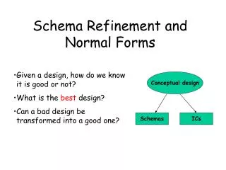
CHAPTER 19 SCHEMA, REFINEMENT AND NORMAL FORMS. INTRODUCTION. Having defined all the relational schemas that we want in our database, the next step is to refine them for so as to (near)optimize them with respect to (memory) space and time (of response to queries).

CHAPTER 19 SCHEMA, REFINEMENT AND NORMAL FORMS
E N D
Presentation Transcript
INTRODUCTION Having defined all the relational schemas that we want in our database, the next step is to refine them for so as to (near)optimize them with respect to (memory) space and time (of response to queries). Much of this optimization can be performed by the optimizer software within the DBMS, but the actual schema cannot be modified by the optimizer, and that is where important improvement can be achieved as we shall find out in this new chapter.
REDUNDANCY AND ITS PROBLEMS (1) Consider the following instance of the Hourly_Emps relation which we have seen earlier: It has been assumed in this relation that the rating implies the hourly wages. This is a special constraint called a functional dependency (FD) which is denoted as follows: rating hourly_wages. As a result of this constraint, the above relation contains a certain amount of redundancy and creates what are called anomalies.
REDUNDANCY AND ITS PROBLEMS (2) - Redundancy: It will be seen, in the above instance, that an hourly_wages of 10 for a rating of 8 is specified three times; similarly an hourly_wages of 7 for a rating of 5 is specified twice. Such redundancy represent wasted memory space i.e. poor design. - Anomalies: There are three kinds of anomalies: (1) Update Anomalies: If we want to change the hourly_wages in the first tuple, we must perform similar changes in the second and fifth tuples. We could specify an integrity constraint for the DBMS to perform such additional changes automatically, but it still requires extra (wasted) time to perform these additional updates. (2) Insertion Anomalies: We cannot insert a (new) employee tuple unless we know the hourly_wages for his rating. (3) Deletion Anomalies: If we delete all tuples with a given rating, we lose the information that this rating corresponds to a certain hourly_wages.
REDUNDANCY AND ITS PROBLEMS (3) The Possibility of Using Null Values - The use of null values cannot resolve the problems of redundant storage and update anomalies. - null value can sometimes help in insertion and delete anomalies, at least when the null value is not forced on a prime key. - Since null values also introduce their own problems it is preferable to avoid them if at all possible.
DECOMPOSITION - All the problems we have described will vanish if we “decompose” our original relation into two relations as shown below: N. B. (1) Note that some extra space is now needed to accommodate the second relation and that the ratings show up in two places, but the net saving in a relation containing some hundreds or thousand of tuples is quite significant. (2) It should be immediately apparent that it is generally more efficient to store entity sets separately from the relations in which they participate, unless certain other constraints are present.
PREVIEW OF THIS CHAPTER Our goal in this chapter is to develop the tools that will (1) permit us to determine when a relational schema is subject to the redundancies and anomalies we have just witnessed. (2) allow us to refine such deficient schema by suitable decomposition, thereby avoiding redundancies and anomalies without loss of information.
THE PROGRAM FOR THIS CHAPTER In order to achieve our stated goals we shall proceed as follows: (1) Define a new type of ICs called Functional Dependencies (FD) which can be used to detect the presence of redundancies and anomalies (R/A) in relational schemas (henceforth we shall simply say schemas). (2) Define a number of normal forms which can be used to classify relations with respect to their liability to incorporate R/A. (3) Introduce a decomposition technique that permits us to replace a relations containing R&A by ‘equivalent’ ones devoid of R/A. (4) Discuss other potential problems (loss of FD characterization) that may plague the resulting relations, and how to deal with such problems
FUNCTIONAL DEPENDENCIES - Functional Dependencies (FDs) are ICs that characterize relations by generalizing the concept of keys. - A functional dependency, X→Y, characterizing a relation R (where X and Y are sets of attributes of R) states that the attribute set Y is completely determined (we say functionally determined) by the attribute set X. - Thus if X is a candidate key (or a superkey) Y is the entire set of attributes of R. - There can be any number and any mixture of FDs that characterize a relation. - The FDs characterizing relations must be specified as part of the semantics of these relations. - The presence of certain FDs in a relation is responsible for the R/A plaguing that relation. - Our job is to locate such FDs and render them harmless.
EXAMPLE OF FUNCTIONAL DEPENDENCIES Consider a relation Contract described by the schema Contracts (contractid, supplierid, projectid, depid, partid, qty, value) and denoted CSJDPQV where the meaning of a tuple is that the contract identified by contractid C is an agreement that supplier S (supplierid) will supply Q items of part P (partid) to project J (projid) associated with department D (deptid), the value V ot this contract being (value). 1. The fact that the key of this relation is C is denoted by the FD C→CSJDPQV which is really an abbreviation for the seven FDs (i) C→C, (ii) C→S, (iii) C→J, (iv) C→D, (v) C→P, (vi) C→Q, (vii) C→V N. B. The FD (i) C→C is called a trivial FD since every attribute is trivially implied by itself. Now suppose we wish to add the following company rules: 2. A project purchases a given part using a single contract: JP→C. 3. A department purchases at most one part from a supplier: SD→P. Thus relation C is characterized by the set of FDs {C→ CSJDPQV, JP→ C, SD→ P}
CLOSURE OF A SET OF FDs: ARMSTRONG AXIOMS - The set of all FDs implied by a given set F of FDs is called the closure of F, denoted F+. - In order to check for the presence of R/A we need to ascertain the possible presence of other FDs implied by those stated explicitly. This means that we have to calculate the closure F+. - This may be done utilizing the Armstrong Axioms which may be stated as follows: letting X, Y, Z denote sets of attributes of a relation R, • Reflexivity: If X⊇Y (i.e. X contains Y) then X→Y. (This rule really generates only trivial FDs). • Augmentation: If X→Y, then XZ→YZ for any Z. • Transitivity: If X→Y and Y→Z, then, X→Z. It may be proven that (1) Armstrong’s axioms are sound, i.e. they generate only FDs in F+. (2)Armstrong’s axioms are complete, i. e. they generate all the FDs in F+. It is convenient to add the following additional rules which may even be considered as denotation rules • Union: If X→Y and X→Z, then X→YZ. • Decomposition: If X→YZ, then X→Y and X→Z. N. B. Note that these axioms do not imply that you may ‘cancel’ attributes appearing on both sides. Thus if AB→ BC, then you may not conclude that A→B.
EXAMPLES OF APPLICATION OF ARMSTRONG AXIOMS (1) Consider the relation ABC with FDs (i) A→B and (ii) B→C. 1. From Reflexivity we get all the trivial FDs which are of the form X→Y, where Y ⊆ X, X ⊆ ABC and Y ⊆ ABC. 2. Applying transitivity to (i) and (ii) we get A → C. 3. From augmentation we get AC → BC, AB → AC, AB →CB. Thus the closure of the set F of given FDs is (apart from trivial FDs): F+ = {A→B, B→C, A → C, AC → BC, AB → AC, AB →CB}
EXAMPLES OF APPLICATION OF ARMSTRONG AXIOMS (2) Consider the previous relation Contracts that is characterized by the set of FDs { (i) C → CSJDPQV, (ii) JP →C, (iii) SD → P}. 1. From (ii), (i), and transitivity we get (iv) JP → CSJDPQV. 2. From (iii) and augmentation we get (v) SDJ → JP. 3. From (v), (iv) and transitivity we get (vi) SDJ → CSDJPQV. 4. From (i) and decomposition we can get C →S, C → J, C → D, C → P,C → Q, C → V. N. B. We have not included trivial dependencies in the above derivations.
ATTRIBUTE CLOSURE Constructing the closure of a set of FDs may be fairly laborious. It may be avoided when one wishes to check what are the possible right-hand sides of an FD X → Y, for a given X, by means of the following algorithm which calculates the so-called attribute closure, denotedX+, of a set X = {A1, A2, … ,An} of attributes, with respect to the set F of FDs. 1. Let X be a set of attributes that eventually will become the closure. First we initialize X to be {A1, A2, … ,An}. 2. We repeatedly search for some FD B1 B2 … Bm→ C such that all of B1 B2 … Bm are in the set of attributes X, but C is not. We then add C to the set X. 3. Repeat step 2 as many times as necessary until no more new attributes can be added to X. 4. The final set X is the correct value of {A1, A2, … ,An}+.
EXAMPLE OF ATTRIBUTE CLOSURE COMPUTATION Given the previous Contracts relation characterized by the FDs (i) C → CSJDPQV, (ii) JP→C, (iii) SD→P Suppose we wish to get the attribute closure of JP, i.e. (JP)+ 1. Initialize the closure (X)+ as {JP}. 2. (i) does not satisfy the requirement that the left side be in JP. (ii) does, therefore we set (X)+ = (X)+ ⋃ C = {JPC}. (iii) does not. We now repeat step 2: 2. (i) now does satisfy the requirement that the left side be in JP, therefore we set (X)+ = (X)+⋃ CSJDPQV = {JPCSDQV}. (ii) and (iii) add nothing new. Repeating step 2 does not change (X)+. Therefore we stop having obtained (JP)+ = {JPCSDQV}+.
NORMAL FORMS (1) The following Normal Forms are used in the RMD to characterize relations: • First Normal Form (1NF). • Second Normal Form (2NF). • Third Normal Form (3NF). • Boyce-Codd Normal Form (BCNF). Later we shall also consider • Fourth Normal Form (4NF) • Fifth Normal Form (5NF)
NORMAL FORMS (2) First Normal Form (1NF) - A relation is said to be in 1NF if it has only single-valued attributes. (This is such a pillar of the RMD that we shall assume it is always true for all the relations we encounter). Second Normal form (2NF) - A relation is said to be in 2NF if it is in 1NF and contains partial dependencies (Actually, 2NF is really of historic interest only). Third Normal Form (3NF) - A relation is said to be in 3NFif it is in 2NF and, for every FD X→A in F, one of the following statements is true: • A∈X; i. e. it is a trivial FD, or • X is a superkey (a superkey is a set of attributes which contains a key), or • A is part of some key for R. Boyce-Codd Normal Form (BCNF) - A relation is said to be in BCNF if it is in 2NF and one of the following two statements is true: • A∈X; i. e. it is a trivial FD, or • X is a superkey.
NORMAL FORMS (3) BCNF The successive containment of Normal Forms may be illustrated by the following diagram: 3NF 2NF 1NF
DIAGRAMATIC VIEW OF FDs PARTIAL DEPENDENCIES IN 2NF, BUT NOT 3NF TRANSITIVE DEPENDENCIES IN 3NF BUT NOT IN BCNF X IS A SUPERKEY IN BCNF
DECOMPOSITION – THE REQUIREMENTS - In order to remove the R/A from a relation it is necessary to decompose it into two or more relations utilizing one of the FDs responsible for the R/A as a ‘pivot point’ of this decomposition. - The decomposition must be lossless, i.e. the final relations must contain exactly the information contained in the original relation, without losing any nor adding any other ones. - The decomposition must be dependency-preserving, i.e. the final relations must be characterized by the same FDs as the original relation so as to permit their verification when modifications are requested. - The above demands lead to the requirement that the final relations be in BCNF if at all possible, or in 3NF otherwise. - We shall now examine some examples drawn from odd-numbered problems in the text.
THE DECOMPOSITION ALGORITHM 1. Check which normal form the relation is in. 2. Locate the FDs responsible for it not being in BCNF. 3. Select one of the responsible FDs. 4. Decompose the relation using the selected responsible FD, say A→B, as the pivot of the decomposition; the decomposition yields two separate relations, say R1 and R2;R1 has for attributes all the attributes occurring in the pivot FD i. e. R1(AB) and no other; R2 has for attributes the set A. 5. Check whether the resulting relations are in BCNF. If they are, go to step 6; otherwise repeat from step 2 on. 6. Check whether the final relations are dependency preserving. If they are, stop; if they are not, you may have several choices: (i) The problem may disappear if you select some alternate responsible FD; try all permissible combinations. (ii) If the problem persist you may choose to leave it in 3NF, or (iii) you may decide to add some other relation to those you have obtained in order to preserve dependencies,
EXAMPLE 1 (19.7-1) Consider a relation R (A B C D) with FDs (i) C → D, (ii) C → A, (iii) B → C - The only candidate key is B. - (i) and (ii) are partial dependencies, so R is not even in 2NF. - pick (ii) as the pivot; the decomposition is now as follows: R (A B C D ) C →A R1(CA) R2(BCD) with C→A with C→D and B→C R2 is not in BCNF decompose with (ii) as pivot. C→D R21(CD) R22(BC) with C→D with B→C R1, R21, and R22 are now in BCNF lossless decomposition and dependencies are preserved.
EXAMPLE 1 (19.7-1) (cont’d) C→D Suppose we now use (i) as the first pivot. We would get R(ABCD) R1(CD) R2(ABC) with C→D with C→A and B→C B→C R21(CA) R22(BC) with C→A with B→C Thus, in this case, the final results are similar.
EXAMPLE 2 (19.7-3) Consider R(ABCD) with (i) ABC→D and (ii) D→A. -The candidate key is (ABC) - R is in 3NF because of (ii) - Decomposing R using (ii) as pivot: R(ABCD) D→A R1(DA) R2(BCD) with D→A The final relations R1 and R2 are both in BCNF. However, the decomposition is not dependency-preserving for FD (i) is not preserved; whenever we make a change in the database we have to re-joinR1 and R2 to be able to verify that (i) is preserved. Therefore we have the following choice: (a) leave R in 3NF as it was originally with its R/A or (b) decompose it into R1 and R2 and join them whenever, there is a change.
EXAMPLE 3 (19.7-5) Consider R(ABCD) with (i) AB→C, (ii) AB→D, (iii) C→A, (iv) D →B - The candidate keys are now AB, BC, CD, AD. - Because of (iii) and (iv), R is in 3NF but not in BCNF. - Decompose using (iii) as pivot: R(ABCD) C→A R1(CA) R2(BCD) with C→A with D→B D→B R21(DB) R22(CD) with D→B The three final relations are in BCNF, but the decomposition is not dependency–preserving since (i) and (ii) cannot be associated with any of the three final relations. The text suggests adding ABC and ABD to R1, R21 and R22. That is an expensive solution!
EXAMPLE 3 (19.10-1) Consider R(ABCD) with (i) B→C, (ii) D→A. Questions: (a) Candidate keys? (b) Is decomposition into BC and AD good or bad? Why? Answers:(a) BD (b) Both (i) and (ii) are partial dependencies. Thus R is in 2NF. Therefore a decomposition is in order. - Following our decomposition algorithm, we should decompose using either (i) or (ii) as pivots. - Using (i) as pivot we get: R(ABCD) B→C R1(BC) R2(ABD) with B→C with D→A D→A This decomposition is good: It is lossless and dependency- preserving. R21(DA) R22(BD) with D→A
EXAMPLE 3 (19.10-1) (cont’d) However, decomposition into BC and AD is unsatisfactory because it is not lossless; it is lossy! Indeed when we join BC and AD we get their cartesian product because they have no attribute in common, and cartesian products are generally much larger than join. Example: Let R= R(BC)= R(AD)= Not equal R(AD) ⋈ R(BC)=
LOSSLESS DECOMPOSITIONS A useful test for lossless decomposition is given in the text by Theorem 3 (p.620):Let R be a relation and F be a set of FDs that hold over R. The decomposition into relations with attribute sets R1 and R2 is lossless if and only if F+ contains either the FD R1∩ R2→ R1 or the FD R1∩ R2 → R2. This theorem yields the following lemma which we have been using in our decomposition: Lemma (p. 620): If an FD X→Y holds over a relation R and X ∩ Yis empty, the decomposition of R into R – Y and XY is lossless. N.B. Do not assume that a lossless decomposition and a decomposition yielding BCNF relations are synonymous.
EXAMPLE 3 (19.10-2) Consider R(ABCD) with (i) AB→C, (ii) C→A, (iii) C→D. Questions: (a) Candidate keys; (b) Is decomposition into R1 = ACD and R2 = BC good or not? Why? Answers: (a) Candidate keys: AB, BC. (b) Consider the losslessness decomposition test: Here R1 = ACD and R2 = BC R1 ∩ R2 = C; thus R1∩ R2 → R1 corresponds to C → ACD which is in F+ since it is derivable from C→C (trivial FD), C→A (ii), C→D (iii). Thus theorem 3 is satisfied and the proposed decomposition is lossless. - Note that this is a BCNF decomposition because: - R1 is characterized by the FDs (ii) C→A and (iii) C→D so that C is the key in R1 and the two FDs follow BCNF requirements. - R2 has the key BC and thus also satisfies BCNF conditions,
EXAMPLE 3 (19.10-2) )cont’d) The decomposition is thus as follows: R(ABCD) with AB→C, C→A, C→D N.B.: No pivot FD. R1(ACD) R2(BC) with C→A and C→D However, the decomposition is not dependency-preserving since the FD AB→C cannot be included in either relation. The text suggests adding the relation ABC to avoid repetitive construction of joins to check for violations of the missing FD.
DEPENDENCY-PRESERVING DECOMPOSITIONS - Definition of the projection of a set F of dependencies: Let R be a relation decomposed into two schemas with attribute sets X and Y, and let F be a set of FDs over R. The projection of F on X is the set of FDs in F+ that involve only attributes in X. It is denoted as FX. - Definition of dependency-preserving decomposition The decomposition of relation R with the set F of FDs into two relations with attribute sets X and Y is dependency-preserving if (FX ⋃ FY)+ = F+ .
ANOTHER LOOK AT DECOMPOSITION So far we have seen lossless-join decomposition that were not dependency-preserving, The opposite can also easily occur: dependency-preserving decomposition which are not lossless-join. Example: Consider the relation R (ABC) with FD A→B. If we decompose it into R1(AB) and R2(BC), we have a dependency-preserving decomposition, however it is not lossless-join. Note that has the key: AC To find a lossless-join decomposition we can use our pivot point algorithm: R(ABC) with A→B A→B R1(AB) R2(AC) with A→B
DECOMPOSITION INTO 3NF (1) The decomposition techniques we have developed for BCNF also work for 3NF. However, here we can develop an algorithm to decompose a relation into a collection of 3NF relations which are both lossless-join and dependency-preserving. The desired algorithm depends on the use of a minimal cover for a set of FDs, which is defined as follows: Definition A minimal cover for a set F of FDs is a set G of FDs such that: 1. Every FD in G is of the form X→A, where A is a single attribute. 2. The closure of F and G are equal F+ = G+ . 3. If we obtain a se H of FDs from G by deleting one or more FDs, or by deleting attributes from an FD in G, then, F+≠ H+.
DECOMPOSITION INTO 3NF (2) Example: Let F = {(i) A→B, (ii) ABCD→E, (iii) EF→G, (iv) EF→H, (v) ACDF→EG}. 1. rewrite (v) as (v) ACDF→E, (vi) ACDF→G. 2. Consider (vi). It is implied by (i), (ii), and (iii) it can be deleted. Similarly we ca delete (v). 3. Consider (ii); since (i) holds, we can replace (ii) with (vii) ACD→E Finally, a minimal cover for F is the set {A→B, ACD→E, EF→G, EF→H}. These operations are easily transformed into an algorithm which appears on p. 626. We can now give an algorithm for putting relations into 3NF with lossless-join and dependency preservation.
DECOMPOSITION INTO 3NF (3) Algorithm for obtaining a lossless-join, dependency preserving decomposition into 3NF relations from a relation R with a set F of FDs that is a minimal cover: Let R1, R2, … , Rn be the desired decomposition where Ri is in 3NF and let Fi denote the projection of F onto the attributes of Ri. 1.Identify the set N of FDs in F that is not preserved, i. e. not included in the closure of the union of Fi’s. 2.For each FD X→A in N, create a relation XA and add it to the decomposition of R.
EXAMPLE OF DEPENDENCY PRESERVATION • Example: • - Consider a relation R (A, B, C) with F = { A B , B C, C A } • Now, we decompose R into two relations R1 and R2 using A B: • R1 (A, B) with FD: A B and R2 (B, C) with FD: B C • Question: Is this decomposition dependency-preserving? • - At first sight, it may appear that the answer is 'no' for the FD, C A, is associated with neither R1 nor R2. • - However, if we apply the test described above, we find • FAB = {A B , B A} and FBC = { B C , C B }, • as the second element in each set is implied by application of transitivity to the original FDs. • Thus, (FAB FBC)+ = F+. Therefore, the decomposition is dependency-preserving. • - But then, where is the FD, C A, in the above decomposition? The answer is that we should have really written the decomposed schemas as: • R1 (A, B) with FAB = { A B, B A} and R2 (B, C) with FBC = { B C, C B} • and C A is automatically preserved when the other FDs are preserved.
NEGATIVE FDs (1) We recall that a ‘negative FD A↛B signifies that the FD A→B is definitely not present. We can use this information as follows: (1) Given a relation R(A1, A2, … , An), draw a list of all possible FDs that might occur in R. This is a rather formidable task, but one can of course write a program to do it. (2) If you are given a whole batch of instances of R, you could write a program to test if these instances contain any negative FDs. (3) If you are trying to set up a database for an organization and the members of the organization do not know (or understand) FDs, You could run a program that generates (minimal) instances where suspected FDs are violated. Showing such instances to the future users often provokes them to realize the presence of FDs that they had not appreciated or realized (“was it not obvious ?”).
NEGATIVE FDs (2) To list all possible FDS in a relation: (1) Relations with 2 attributes R(AB): [3 possibilities] R(AB) A→B; R(AB) B→A; R(AB) A→B & B→A. (Thus always in BCNF) (2) Relations with 3 attributes R(ABC): (i) 1 FD: A→B; A→C; B→C; B→A; C→A; C→B; AB→C; AC→B; BC→A. [9] (ii) 2 FDs: A→B & A→C; A→B & B→C; A→B & B→A; A→B & C→A; A→B & C→B; A→B & AB→C; A→B & AC→B; A→B & BC→A. [8] A→C & B→C; A→C & B→A; AC & C→A; A→C & C→B; A→C & AB→C; A→C & AC→B; A→C & BC→A. [7] B→C & B→A; B→C & … [6] B→A & C→A; B→A & … [5] C→A & C→B; C→A & … [4] C→B & AB→C; … [3] AB→C & AC→B; … [2] AC→B & BC→A; … [1] So far 9 + 8 +7 +6 + 5 +4 +3 +2 +1 = 45
NEGATIVE FDs (3) (iii) 3FDs: A→B & A→C & B→C; … [7] A→B & B→C & B→A; … [6 ] A→B & B→A & C→A; … [5] A→B & C→A & C→B; … [4] A→B & C→B & AB→C; … [3] A→B & AB→C & AC→B; … [2] A→B & AC→B & BC→A; … [1] adding up to 28 ADDING UP TO 459 = 405 “ 405 + 45 + 9 = 459 (NO GUARANTEE)
MULTIVALUED DEPENDENCIES C/T/B The meaning of a tuple is that teacher T can teach course C, and book B is a recommended text for the course. However, the recommended texts for a course are independent of the instructor, an IC which cannot be expressed in terms of FDs.
MVDs and the ER Model The presence of MVDs in our initial Course/Teachers/Books relation may be seen in the ER model as an inappropriate attempt to use a ternary relationship set in stead of two binary relationship sets: books teachers C/B/T courses C/T teachers courses books C/B
MVDs DECOMPOSITION C/B C/T The Redundancies will be removed if we decompose as follows: The redundancy problem was due to the fact that we were trying to put into a single relation two completely separate kinds of data. That is the source of MVDs.
MULTIVALUED DEPENDENCIES DEFINITION tuple names tuple names
Thus, according to definition: C→→T iff t1.C = t2.C = Physics and ∃ t3 such that t1.CT= t3.CT = Physics/Green & t2.B = t3.B = Optics Similarly there must exist a t4 such that t2.CT = t4.CT t1.B = t4.B = Mechanics C→→T Thus, for every teacher, there must be thesame set of books, namely Optics and Mechanics. MVD – APPLICATION OF DEFINITION (1) N. B. (1) I have rearranged the rows of the original instance so that they fit the formal definition. (2) If the were n books used in the Physics course, then there would have to be n tuples for each teacher in order for the MVD to hold. Similarly, if there were m teachers, then there would have to be m tuples for each book in order for the MVD to hold. (3) The the last three rows cannot be used to verify the presence of MVD.
MVD – APPLICATION OF DEFINITION (1) A similar analysis shows that there must also be a ‘paired’ MVD, C→→B: Thus, according to definition: C→→B iff When t1.C = t2.C = Physics and there exists a t2 such that t1.CB = t2.CB = Physics/Mechanics & t1.T = t3.T = Green & there exists a t4 such that t1.CB = t4.CB = Physics/Optics & t1.T = t4.T = Brown & there exists as many tn as
A BETTER DEFINITION TO TEST FOR MVDs We can always test for the presence of MVD utilizing the following definition: Given a relation R and attribute sets X, Y, Z with Z = R ╸XY, then the MVD X→→Y holds over R if, for any legal instance over R, for any value x that appears in the X column of R, πYZ (σX=x(R)) =πY(σX=x(R) πZ(σX=x(R)) N.B. The following examples are much better understood in terms of this relation as described in class. Students should practice its usage through those examples.
MVD – APPLICATION OF DEFINITION (2) Applying to the first 4 rows (X=Physics) the condition: X→→Y if πYZ (σX=x(R)) =πY(σX=x(R) πZ(σX=x(R)) for X = C, Y = T, Z = B, =P yields: σX=x(R) = {<P, G, m>, <P, G, o>, <P, B, m>, <P, B, o>} and πYZ (σX=x(R)) = {<G, m>, <G, o>, <B, m>, <B, o>} πY(σX=x(R) πZ(σX=x(R)) = {<G>, <B>} {m>, <o>} = {<G, m>, <G, o>, <B, m>, <B, o>} Applying the same condition to the last 3 rows (X= Math) yields: σX=x(R) = {<M, G, m>, <M, G, v>, <M, G, g>} πYZ (σX=x(R)) = {<G, m>, <G, v>, <G, g>} πY(σX=x(R) πZ(σX=x(R)) = {<G>} {<m>, <v>, <g>} = {<G, m>, <G, v>, <G, g>} Therefore the MVD conditions hold. = =
MVD – APPLICATION OF DEFINITION (3) Same sets t1 t3 t4 t2 t1 t4 t3 `t2 Same sets Consider the CBT relation If there is an MVD C →→ T, then, for every course such as Physics 101 that is taught by any teacher (here Green and Brown), the same set of books must be recommended (Mechanics and Optics). There must also be an MVD C →→ B, whereby, for every course such as Physics 101 for any book that is recommended (here Mechanics and Optics), the same set of teachers must be shown for this course (Green and Brown).
A SOUND AND COMPLETE SET OF INFERENCE RULES FOR FDs AND MVDs Given a set of FDs and MVDs we can infer all of them by using Armstrong Axioms plus the following five rules: • MVD Complementation: If X →→ Y, then X →→ ( R ╸XY). • MVD Augmentation: If X →→ Y and W ⊇ Z, then WZ →→ YZ. • MVD Transitivity: If X →→ Y and Y →→ Z, then X →→ Z. • Replication: If X → Y, then X →→ Y. (Every FD is an MVD) • Coalescence: If X →→ Y and there is a W such that W ∩ Y = φ, W → Z, and Y ⊇ Z, then X →→ Z. N.B.: Note that according to MVD Complementation MVDs always occur in pairs.