Schema Refinement and Normal Forms
Schema Refinement and Normal Forms. Chapter 19. Instructor: Mirsad Hadzikadic. The Evils of Redundancy. Redundancy is at the root of several problems associated with relational schemas: redundant storage, insert/delete/update anomalies

Schema Refinement and Normal Forms
E N D
Presentation Transcript
Schema Refinement and Normal Forms Chapter 19 Instructor: Mirsad Hadzikadic
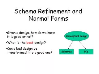
The Evils of Redundancy • Redundancyis at the root of several problems associated with relational schemas: • redundant storage, insert/delete/update anomalies • Integrity constraints, in particularfunctional dependencies, can be used to identify schemas with such problems and to suggest refinements. • Main refinement technique: decomposition (replacing ABCD with, say, AB and BCD, or ACD and ABD). • Decomposition should be used judiciously: • Is there a reason to decompose a relation? • What problems (if any) does the decomposition solve?
Functional Dependencies (FDs) • A functional dependencyX Y holds over relation R if, for every allowable instance r of R: • t1 r, t2 r, (t1) = (t2) implies (t1) = (t2) • i.e., given two tuples in r, if the X values agree, then the Y values must also agree. (X and Y are sets of attributes.) • An FD is a statement about all allowable relations. • Must be identified based on semantics of enterprise. • Given some allowable instance r1 of R, we can check if it violates some FD f, but we cannot tell if f holds over R!
Example: Constraints on Entity Set • Consider relation obtained from Hourly_Emps: • Hourly_Emps (ssn, name, lot, rating, hrly_wages, hrs_worked) • Notation: We will denote this relation schema by listing the attributes: SNLRWH • This is really the set of attributes {S,N,L,R,W,H}. • Sometimes, we will refer to all attributes of a relation by using the relation name. (e.g., Hourly_Emps for SNLRWH) • Some FDs on Hourly_Emps: • ssn is the key: S SNLRWH • rating determines hrly_wages: R W
Example (Contd.) • Problems due to R W : • Update anomaly: Can we change W in just the 1st tuple of SNLRWH? • Insertion anomaly: What if we want to insert an employee and don’t know the hourly wage for his rating? • Deletion anomaly: If we delete all employees with rating 5, we lose the information about the wage for rating 5! Hourly_Emps2 Wages
Reasoning About FDs • Given some FDs, we can usually infer additional FDs: • ssn did, did lot implies ssn lot • An FD f is implied bya set of FDs F if f holds whenever all FDs in F hold. • = closure of F is the set of all FDs that are implied by F. • Armstrong’s Axioms (X, Y, Z are sets of attributes): • Reflexivity: If X Y, then X Y • Augmentation: If X Y, then XZ YZ for any Z • Transitivity: If X Y and Y Z, then X Z • These are sound and completeinference rules for FDs!
Reasoning About FDs (Contd.) • Couple of additional rules : • Union: If X Y and X Z, then X YZ • Decomposition: If X YZ, then X Y and X Z
Example • A relation R has attributes (S, C, T, R, G) which denotes student, course, time, room, and grade respectively. From requirements, the following FDs hold. • SC G • ST R • C T • TR C
Attribute Closure • Computing the closure of a set of FDs can be expensive. (Size of closure is exponential in # attrs!) • Typically, we just want to check if a given FD X Y is in the closure of a set of FDs F. An efficient check: • Compute attribute closureof X (denoted ) wrt F: • Set of all attributes A such that X A is in • There is a linear time algorithm to compute this. • Check if Y is in
Attribute Closure • Algorithm • Closure = X; • Repeat until there is no change{ • If there is an FD in F such that U closure • Then set closure = closure V }
Example 2 • A relation R has attributes (A,B,C,D,E) with FDs • AB • BCE • EDA Compute all keys for R
Normal Forms • Returning to the issue of schema refinement, the first question to ask is whether any refinement is needed! • If a relation is in a certain normal form(BCNF, 3NF etc.), it is known that certain kinds of problems are avoided/minimized. This can be used to help us decide whether decomposing the relation will help. • The role of FDs in detecting redundancy: • Consider a relation R with 3 attributes, ABC. • No FDs hold: There is no redundancy here. • Given A B: Several tuples could have the same A value, and if so, they’ll all have the same B value!
Boyce-Codd Normal Form (BCNF) • Reln R with FDs F is in BCNF if, for all X A in • A X (called a trivial FD), or • X contains a key for R. • In other words, R is in BCNF if the only non-trivial FDs that hold over R are key constraints. • No redundancy in R that can be predicted using FDs alone. • If example relation is in BCNF, the 2 tuples must be identical (since X is a key).
Third Normal Form (3NF) • Reln R with FDs F is in 3NF if, for all X A in • A X (called a trivial FD), or • X contains a key for R, or • A is part of some key for R. • Minimality of a key is crucial in third condition above! • If R is in BCNF, obviously in 3NF. • If R is in 3NF, some redundancy is possible. It is a compromise, used when BCNF not achievable (e.g., no “good’’ decomp, or performance considerations). • Lossless-join, dependency-preserving decomposition of R into a collection of 3NF relations always possible.
What Does 3NF Achieve? • If 3NF violated by X A, one of the following holds: • X is a subset of some key K • We store (X, A) pairs redundantly. • X is not a proper subset of any key. • There is a chain of FDs K X A, which means that we cannot associate an X value with a K value unless we also associate an A value with an X value.
Decomposition of a Relation Scheme • Suppose that relation R contains attributes A1 ... An. A decompositionof R consists of replacing R by two or more relations such that: • Each new relation scheme contains a subset of the attributes of R (and no attributes that do not appear in R), and • Every attribute of R appears as an attribute of one of the new relations. • Intuitively, decomposing R means we will store instances of the relation schemes produced by the decomposition, instead of instances of R. • E.g., Can decompose SNLRWH into SNLRH and RW.
Example Decomposition • Decompositions should be used only when needed. • SNLRWH has FDs S SNLRWH and R W • Second FD causes violation of 3NF; W values repeatedly associated with R values. Easiest way to fix this is to create a relation RW to store these associations, and to remove W from the main schema: • i.e., we decompose SNLRWH into SNLRH and RW • The information to be stored consists of SNLRWH tuples.
Problems with Decompositions • There are three potential problems to consider: • Some queries become more expensive. • e.g., How much did sailor Joe earn? (salary = W*H) • Given instances of the decomposed relations, we may not be able to reconstruct the corresponding instance of the original relation! • Fortunately, not in the SNLRWH example. • Checking some dependencies may require joining the instances of the decomposed relations. • Fortunately, not in the SNLRWH example. • Tradeoff: Must consider these issues vs. redundancy.
Lossless Join Decompositions • Decomposition of R into X and Y is lossless-join w.r.t. a set of FDs F if, for every instance r that satisfies F: • (r) (r) = r • Definition extended to decomposition into 3 or more relations in a straightforward way. • It is essential that all decompositions used to deal with redundancy be lossless! (Avoids Problem (2).)
More on Lossless Join • The decomposition of R into X and Y is lossless-join wrt F if and only if the closure of F contains: • X Y X, or • X Y Y • In particular, the decomposition of R into UV and R - V is lossless-join if U V is empty and U V holds over R. Not a Lossless Join
Dependency Preserving Decomposition • Consider CSJDPQV, C is key, JP C and SD P. • BCNF decomposition: CSJDQV and SDP • Problem: Checking JP C on tuple insert requires a join! • Dependency preserving decomposition (Intuitive): • If R is decomposed into X, Y and Z, and we enforce the FDs that hold on X, on Y and on Z, then all FDs that were given to hold on R must also hold. (Avoids Problem (3).)
Decomposition into BCNF • Consider relation R with FDs F. If X Y violates BCNF and Y is single attribute, decompose R into R - Y and XY. • Repeated application of this idea will give us a collection of relations that are in BCNF; lossless join decomposition, and guaranteed to terminate. • e.g., CSJDPQV, key C, JP C, SD P, J S • To deal with SD P, decompose into SDP, CSJDQV. • To deal with J S, decompose CSJDQV into JS and CJDQV • In general, several dependencies may cause violation of BCNF. The order in which we ``deal with’’ them could lead to very different sets of relations!
BCNF and Dependency Preservation • In general, there may not be a dependency preserving decomposition into BCNF. • e.g., CSZ, CS Z, Z C • Can’t decompose while preserving 1st FD; not in BCNF. • Similarly, decomposition of CSJDQV into SDP, JS and CJDQV is not dependency preserving (w.r.t. the FDs JP C, SD P and J S). • However, it is a lossless join decomposition. • In this case, adding JPC to the collection of relations gives us a dependency preserving decomposition. • JPC tuples stored only for checking FD! (Redundancy!)
Decomposition into 3NF • Obviously, the algorithm for lossless join decomp into BCNF can be used to obtain a lossless join decomp into 3NF (typically, can stop earlier). • To ensure dependency preservation, one idea: • If X Y is not preserved, add relation XY. • Problem is that XY may violate 3NF! e.g., consider the addition of CJP to `preserve’ JP C.
Summary of Schema Refinement • If a relation is in BCNF, it is free of redundancies that can be detected using FDs. Thus, trying to ensure that all relations are in BCNF is a good heuristic. • If a relation is not in BCNF, we can try to decompose it into a collection of BCNF relations. • Must consider whether all FDs are preserved. If a lossless-join, dependency preserving decomposition into BCNF is not possible (or unsuitable, given typical queries), should consider decomposition into 3NF. • Decompositions should be carried out and/or re-examined while keeping performance requirements in mind.
Normal Form • Example • A company obtains parts from a number of suppliers. • Each supplier is located in one city. • A city can have more than one supplier located there • and each city has a status code associated with it. • Each supplier may provide many parts.
First normal form • All values of the columns are atomic
Anomalies with 1NF • INSERT. • The fact that a certain supplier (s5) is located in a particular city (Athens) cannot be added until they supplied a part. • DELETE. • If a row is deleted, then not only is the information about quantity and part lost but also information about the supplier. • UPDATE. • If supplier s1 moved from London to New York, then six rows would have to be updated with this new information.
2NF • A relational table is in second normal form 2NF if it is in 1NF and every non-key column is fully dependent upon the primary key. • Is FIRST in 2NF? • S#->city,status • City->status • (s#,p#)->qty
Decompose 1NF into 2NF • Identify any determinants other than the composite key, and the columns they determine. • Create and name a new table for each determinant and the unique columns it determines. • Move the determined columns from the original table to the new table. The determinate becomes the primary key of the new table. • Delete the columns you just moved from the original table except for the determinate which will serve as a foreign key. • The original table may be renamed to maintain semantic meaning.
Problems of 2NF • INSERT. • The fact that a particular city has a certain status (Rome has a status of 50) cannot be inserted until there is a supplier in the city. • DELETE. • Deleting any row in SUPPLIER destroys the status information about the city as well as the association between supplier and city.
3NF • A relational table is in third normal form (3NF) if it is already in 2NF and every non-key column is non transitively dependent upon its primary key. In other words, all nonkey attributes are functionally dependent only upon the primary key. • SUPPLIER is in 2NF but not in 3NF because it contains a transitive dependency. • A transitive dependency occurs when a non-key column that is a determinant of the primary key is the determinate of other columns.
Decompose to 3NF • Identify any determinants, other the primary key, and the columns they determine. • Create and name a new table for each determinant and the unique columns it determines. • Move the determined columns from the original table to the new table. The determinate becomes the primary key of the new table. • Delete the columns you just moved from the original table except for the determinate which will serve as a foreign key. • The original table may be renamed to maintain semantic meaning.
Advantages of 3NF • it eliminates redundant data • INSERT. • Facts about the status of a city, Rome has a status of 50, can be added even though there is not supplier in that city. • Likewise, facts about new suppliers can be added even though they have not yet supplied parts. • DELETE. • Information about parts supplied can be deleted without destroying information about a supplier or a city. • UPDATE. • Changing the location of a supplier or the status of a city requires modifying only one row.
Advanced NFs • After 3NF, all normalization problems involve only tables which have three or more columns and all the columns are keys. • Many practitioners argue that placing entities in 3NF is generally sufficient because it is rare that entities that are in 3NF are not also in 4NF and 5NF. • They further argue that the benefits gained from transforming entities into 4NF and 5NF are so slight that it is not worth the effort.
BCNF • Boyce-Codd normal form (BCNF) is a more rigorous version of the 3NF deal with relational tables that had (a) multiple candidate keys, (b) composite candidate keys, and (c) candidate keys that overlapped . • BCNF is based on the concept of determinants. A determinant column is one on which some of the columns are fully functionally dependent. • A relational table is in BCNF if and only if every determinant is a candidate key.
4NF • A relational table is in the fourth normal form (4NF) if it is in BCNF and all multivalued dependencies are also functional dependencies. • Multi-valued dependencies • given a relational table R with columns A, B, and C then R.A —>> R.B (column A multidetermines column B) is true if and only if the set of B-values matching a given pair of A-values and C-values in R depends only on the A-value and is independent of the C-value. • MVD always occur in pairs. That is R.A —>> R.B holds if and only if R.A —>> R.C also holds.
Examples • employees can be assigned to multiple projects and employees can have multiple job skills. • The primary key should be (emp#,prj#,skill#) • The relationship between emp# and prj# is a multivalued dependency because for each pair of emp#/skill values in the table, the associated set of prj# values is determined only by emp# and is independent of skill. • The relationship between emp# and skill is also a multivalued dependency, since the set of Skill values for an emp#/prj# pair is always dependent upon emp# only.
5NF • A table is in the fifth normal form (5NF) if it cannot have a lossless decomposition into any number of smaller tables. • http://www.utexas.edu/cc/database/datamodeling/rm/rm7.html • http://www.utexas.edu/cc/database/datamodeling/rm/rm8.html