Statistical Analysis of Microarray Data

1. Statistical Analysis of Microarray Data Ka-Lok Ng

2. Statistical Analysis of Microarray Data Ratios and reference samples • Compute the ratio of fluorescence intensities for two samples that are competitively hybridized to the same microarray. One sample acts as a control , or “reference” sample, and is labeled with a dye (Cy3) that has a different fluorescent spectrum from the dye (Cy5) used to label the experimental sample. • A convention emerged that two-foldinduction or repression of an experimental sample, relative to the reference sample, were indicative of a meaningful change in gene expression. • This convection does not reflect standard statistical definition of significance • This often has the effect of selecting the top 5% or so of the clones present on the microarray

3. Statistical Analysis Microarray Data Reasons for adopting ratios as the standard for comparison of gene expression • Microarrays do not provide data on absolute expression levels. Formulation of a ratio captures the central idea that it is a change in relative level of expression that is biological interesting. • removes variation among arrays from the analysis. Differences between microarray – such as (1) the absolute amount of DNA spotted on the arrays, (2) local variation introduced either during the sliding preparation and washing, or during image capture.

4. Simple normalization of microarray data. The difference between the raw fluorescence is a meaningless number. Computingratiosallows immediate visualization of which genes are higher in the red channel than the green channel, but logarithmic transformation of this measure on the base 2 scale results in symmetric distribution of values. Finally, normalization by subtraction of the mean log ratio adjusts for the fact that the red channel was generally more intense than the green channel, and centers the data around zero. Statistical Analysis of Microarray Data All microarray experiments must be normalized to ensure that biases inherent in each hybridization are removed. True whether use ratios or raw fluorescent intensities are adopted as the measure of transcript abundance.

5. Statistical Analysis of Microarray Data

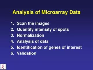
6. Calculate which genes are differentially expressed. Statistical Analysis of Microarray Data Calculate which genes are differentially expressed The fluorescence intensity for the Cy3 or Cy5 channel after background subtraction. Calculate which genes are at least twofold different in their abundance on this array using two different approaches: (a) by formulating the Cy3:Cy5 ratio, and (b) by calculating the difference in the log base 2 transformed values. In both cases, make sure that you adjust for any overall difference in intensity for the two dyes and comment on whether this adjustment affects your conclusions.

7. Statistical Analysis of Microarray Data Divide by 0.954

8. Statistical Analysis of Microarray Data Using the ratio method, without adjustment for overall dye effects, genes 2 and 9 appear to have Cy3/Cy5 < 0.5, suggesting that they are differentially regulated. No genes have Cy3/Cy5 > 2. However, the average ratio is 0.95, indicating that overall fluorescence is generally 5% greater in the Cy5 (RED) channel. One way to adjust for this is to divide the individual ratios by the average ratio, which results in the adjusted ratio column. This confirm that gene 2 is underexpressed in Cy3, but not gene 9, whereas gene 5 may be overexpressed.

9. Statistical Analysis of Microarray Data Using the log transformation method, you get very similar results(-1 and +1). The adjusted columns indicate the difference between the log2 fluorescenec intensity and the mean log2 intensity for the respective dye, and hence express the relative fluorescence intensity, relative to the sample mean. The difference between these values gives the final column, indicating that genes 2 and 5 may differentially expressed by twofold or more.

10. Statistical Analysis of Microarray Data If you just subtract the raw log2 values, you will see that gene 9 appears to be underexpressed in Cy3, but gene 5 appears to be slightly less than twofold overexpressed.

11. Finding significant genes • After normalizing, filtering and averaging the data, one can identify genes with expression ratios that are significantly different from 1 or -1 • Some genes fluctuates a great deal more than others (Hughes et al. 2000a, b) • In general the genes whose expression is most variable are those in which expression is stress induced, modulated by the immune system or hormonally regulated (Pritchard et al. 2001) • There is the Missing Value problem in microarray data set • By interpolation • References • Hughes TR, et al. (2000a) Functional discovery via a compendium of expression profiles. Cell 102(1):109-26 • Hughes TR, et al. (2000b) Widespread aneuploidy revealed by DNA microarray expression profiling. Nat Genet 25(3):333-7 • Pritchard et al. 2001 Project normal: Defining normal variance in mouse gene expression. PNAS 98, 13266.

12. Measure of similarity – definition of distance A measure of similarity - distance • Euclidean distance between two genes • for example: p53 and mdm2

13. Measure of similarity – definition of distance Non-Euclidean metrics • Any distance dijbe the distance between two vectors, i and j must satisfy a number of rules: • The distance must be positive definite • The distance must be symmetric, dij = dji • An object is zero distance from itself, dii =0 • Triangle inequality dik ≦ dij + djk • Manhattan distance (or city block) distance is an example of non-Euclidean distance metric, The Mahattan distance is defined as the sum of the absolute distances between the components of each expression vector, x and y, It measures the route one might have to travel between two points in a place such as Manhattan where the streets and avenues are arranged at right angles to one another. It is known as Hamming distance when applied to data expressed in binary form, e.g. if the expression levels of the genes have been discretised into 1s and 0s.

14. Measure of similarity – definition of distance • Minkowski distance is a generalization of the Euclidean distance and is expressed as The parameter p is called the order. The higher the value of p, the more significant is the contribution of the largest components |ai – bi |. p=1  Manhattan distance p=2  Euclidean distance Herman Minkowski (1864-1909) http://library.thinkquest.org/05aug/01273/whoswho.html

15. A B chord distance angular distance Measure of similarity – definition of distance • Euclidean distance is one of the most intuitive ways to measure the distance between points in space, but it is not always the most appropriate one for expression profiles. • We need to define distance measures that score as similar gene expression profiles that show similar trend, rather than those that depend on the absolute levels. • Two simple measures that can be used are the angle and chord distances. A B chord distance angular distance

16. A B B chord distance angular distance Measure of similarity – definition of distance • A = (ax, ay), B = (bx, by) • The cosine of the angle between the two vectors A and B is given by their dot product, and can be used as a similarity measure. In n-dimensional space for vectors A = (a1, …. an) and B = (b1, …. bn), the cosine is defined as The chord distance is defined as the length of the chord between the vectors of unit length having the same directions as the original ones.

17. Semimetric distance – Pearson correlation coefficient or Covariance Statistics – standard deviation and variance, var(X)=s2, for 1-dimension data • How about higher dimension data ? • It is useful to have a similar measure to find out how much the • dimensions vary from the mean with respect to each other. • Covariance is measured between 2 dimensions, • suppose one have a 3-dimension data set (X,Y,Z), then one can • calculate Cov(X,Y), Cov(X,Z) and Cov(Y,Z) - to compare heterogenous pairs of variables, define the correlation coefficient or Pearson correlation coefficient, -1≦rXY ≦1 -1  perfect anticorrelation 0  independent +1 perfect correlation

18. Semimetric distance – Pearson correlation coefficient or Covariance • The resulting rXYvalue will be larger than 0 if a and b tend to increase • together, below 0 if they tend to decrease together, and 0 if they are • independent. • Remark:rXYonly test whether there is a lineardependence, Y=aX+b • if two variables independent  low rXY, • a low rXYmay or may not independent, it may be a non-linear relation • a high rXYis a sufficient but not necessary condition for variable dependence

19. Semimetric distance – Pearson correlation coefficient or Covariance matrix A covariance matrix is merely collection of many covariances in the form of a d x d matrix:

20. Semimetric distance – the squared Pearson correlation coefficient • Pearson correlation coefficient is useful for examining correlations in the data, but not useful for identifying genes whose expression levels are anticorrelated. • One may imagine an instance, for example, in which the same TF can cause both enhancement and repression of expression. • A better alternative is the squared Pearson correlation coefficient (pcc), The square pcc takes the values in the range 0 ≦ rsq ≦ 1. 0  uncorrelate vector 1  perfectly correlated or anticorrelated pcc are measures of similarity Similarity and distance have a reciprocal relationship similarity↑  distance↓  d = 1 – r is typically used as a measure of distance

21. Statistical Analysis of Microarray Data • Normalize each channel separately  Gn-<G> and Rn-<R> • Subtraction of the mean log fluorescence intensity for the channel from each value transforms the measurements such that the abundance of each transcript is represented as a fold increase or decrease relative to the sample mean, namely as a relative fluorescence intensity. • Log Gn - <log Gn>,Log Rn - <log Rn>, where n=1,2,…. and

22. Statistical Analysis of Microarray Data