Efficient Parallel Computations: Master-Slave Organization for Geometrical Transformations and Mandelbrot Set Analysis
Learn about ideal parallel computation models focusing on minimal interactions and efficient load balancing. Dive into examples of geometric image transformation algorithms, from shifting to rotation and clipping. Discover the Mandelbrot set analysis, exploring quasi-stable points in the plane through iterative functions. Understand static task assignment in parallel processing for optimized performance.

Efficient Parallel Computations: Master-Slave Organization for Geometrical Transformations and Mandelbrot Set Analysis
E N D
Presentation Transcript
Embarrassingly Parallel Computations Chapter 3
1. Ideal Parallel Computation • In this chapter, we will consider applications where there is minimal interaction between the slave processes. • Slaves may be statically assigned or dynamically assigned. • Load balancing techniques can offer improved performance. • We will introduce simple load balancing here • Chapter 7 will cover load balancing when the slaves must interact.
1. Ideal Parallel Computation • Parallelizing these should be obvious and requires no special techniques or algorithms. • A truly embarrassingly parallel computation requires no communication. (SPMD Model)
1. Ideal Parallel Computation • Nearly embarrassingly parallel computations • Require results to be distributed and collected in some way. • A common approach is the Master-Slave organization.
2. Embarrassingly Parallel Examples • 2.1 Geometrical Transformation of Images • The most basic way to store a computer image is a pixmap (each pixel is stored in a 2D array) • Geometrical transformations require mathematical operations to be performed on the coordinates of each pixel without affecting its value.
2.1 Geometrical Transformation of Images • There are several different transformations • Shifting • Object is shifted Dx in the x dimension and Dy in the y dimension: • x’=x+ Dx • y’=y+ Dy • Where x and y are the original and x’ and y’ are the new coordinates. • Scaling • Object scaled by factor Sx in the x-direction and Sy in the y-direction • x’=xSx • y’=ySy
2.1 Geometrical Transformation of Images • Rotation • Object rotated through an angle q about the origin of the coordinate system: • x’=x cosq + y sinq • y’=-x sinq + y cosq • Clipping • Deletes from the displayed picture those points outside the defined area.
2.1 Geometrical Transformation of Images • The input data is the pixmap (bitmap) • Typically held in a file, then copied into an array. • The master is concerned with dividing up the array among the processors. • There are two methods: • Blocks • Stripes
2.1 Geometrical Transformation of Images: Master – pseudo code for (i = 0, row = 0; i < 48; i++, row = row + 10) /* for each process*/ send(row, Pi); /* send row no.*/ for (i = 0; i < 480; i++) /* initialize temp */ for (j = 0; j < 640; j++) temp_map[i][j] = 0; for (i = 0; i < (640 * 480); i++) { /* for each pixel */ recv(oldrow,oldcol,newrow,newcol, PANY); /* accept new coords */ if !((newrow < 0)||(newrow >= 480)||(newcol < 0)||(newcol >= 640)) temp_map[newrow][newcol]=map[oldrow][oldcol]; } for (i = 0; i < 480; i++) /* update bitmap */ for (j = 0; j < 640; j++) map[i][j] = temp_map[i][j];
2.1 Geometrical Transformation of Images: Slave – pseudo code recv(row, Pmaster); /* receive row no. */ for (oldrow = row; oldrow < (row + 10); oldrow++) for (oldcol = 0; oldcol < 640; oldcol++) {/* transform coords */ newrow = oldrow + delta_x; /* shift in x direction */ newcol = oldcol + delta_y; /* shift in y direction */ send(oldrow,oldcol,newrow,newcol, Pmaster);/* coords to master */ }
2.1 Geometrical Transformation of Images: Analysis • Sequential: If each pixel required 1 time step then • ts = n2 • So, time complexity is O(n2) • Recall that for parallel • tp = tcomp + tcomm • tcomm = tstartup + mtdata =O(m) • tcomp = 2(n2/p) = O(n2/p) • tp = O(n2) • What’s the problem?
2.1 Geometrical Transformation of Images: Analysis • The constants for the communication (for parallel) far exceed the constants in the computation (for sequential) • Makes it relatively impractical • This problem is probably better suited for a shared memory system.
2.2 Mandelbrot Set • Def: set of points in the plane that are quasi-stable when computed by iterating the function: • zk+1 = zk2+c • Note: • z is complex, and c is complex. • The initial value for z is 0 • Iterations continue until • the magnitude of z is greater than 2 • or the number of iterations reaches some limit
2.2 Mandelbrot Set: Sequential int cal_pixel(complex c) { int count, max; complex z; float temp, lengthsq; max = 256; z.real = 0; z.imag = 0; count = 0; /* number of iterations */ do { temp = z.real * z.real - z.imag * z.imag + c.real; z.imag = 2 * z.real * z.imag + c.imag; z.real = temp; lengthsq = z.real * z.real + z.imag * z.imag; count++; } while ((lengthsq < 4.0) && (count < max)); return count; }
2.2 Mandelbrot Set: Parallel • Static Task Assignment – Master for (i = 0, row = 0; i < 48; i++, row = row + 10) /* for each process*/ send(&row, Pi); /* send row no.*/ for (i = 0; i < (480 * 640); i++) { /* from processes, any order */ recv(&c, &color, PANY); /*receive coords & colors */ display(c, color); /* display pixel on screen */ }
2.2 Mandelbrot Set: Slave recv(&row, Pmaster); /* receive row no. */ for (x = 0; x < disp_width; x++) /* screen coordinates x and y */ for (y = row; y < (row + 10); y++) { c.real = min_real + ((float) x * scale_real); c.imag = min_imag + ((float) y * scale_imag); color = cal_pixel(c); send(&c, &color, Pmaster);/* send coords, color to master */ }
2.2 Mandelbrot Set • Dynamic Task Assignment • Work Pool/Processor Farms
Master count = 0; /* counter for termination*/ row = 0; /* row being sent */ for (k = 0; k < procno; k++) { /* assuming procno<disp_height */ send(&row, Pk, data_tag); /* send initial row to process */ count++; /* count rows sent */ row++; /* next row */ } do { recv (&slave, &r, color, PANY, result_tag); count--; /* reduce count as rows received */ if (row < disp_height) { send (&row, Pslave, data_tag); /* send next row */ row++; /* next row */ count++; } else send (&row, Pslave, terminator_tag); /* terminate */ rows_recv++; display (r, color); /* display row */ } while (count > 0);
2.2 Mandelbrot Set: Slave recv(y, Pmaster, ANYTAG, source_tag); /* receive 1st row to compute */ while (source_tag == data_tag) { c.imag = imag_min + ((float) y * scale_imag); for (x = 0; x < disp_width; x++) { /* compute row colors */ c.real = real_min + ((float) x * scale_real); color[x] = cal_pixel(c); } send(&i, &y, color, Pmaster, result_tag); /* row colors to master */ recv(y, Pmaster, source_tag); /* receive next row */ };
2.2 Mandelbrot Set: Analysis • Sequential • ts= max x n = O(n) • Parallel • Phase 1: Communication Out • tcomm=s(tstartup+tdata) • It could be possible to use a scatter routine here which would cut the number of startup times. • Phase 2: Computation • (max x n)/s • Phase 3: Communication Back in • tcomm2= (n/s)(tstartup+tdata) • Overall • tp <= (max x n)/s + (n/s + s)(tstartup+tdata)
2.3 Monte Carlo Methods • The basis of Monte Carlo methods is the use of random selections in calculations. • Example – Calculate p • A circle is formed within a square • The circle has unit radius • Therefore the square has sides of length 2 • Area of the square is 4
2.3 Monte Carlo Methods • The ratio of the area of the circle to the square is • (p r2)/2x2 = p/4 • Points within the square are chosen randomly and a score is kept of how many points happen to lie within the circle • The fraction of points within the circle will be p/4, given a sufficient number of randomly selected samples.
2.3 Monte Carlo Methods • Random Number Generation • The most popular way of creating a pueudorandom number sequence: • x1, x2, x3, …, xi-1, xi, xi+1, …, xn-1, xn, • is by evaluating xi+1 from a carefully chosen function of xi, often of the form • xi+1 = (axi+ c) mod m • where a, c, and m are constants chosen to create a sequence that has similar properties to truly random sequences.
2.3 Monte Carlo Methods • Parallel Random Number Generation • It turns out that • xi+1 = (axi+ c) mod m • xi+k= (Axi+ C) mod m • where • A = akmod m, • C = c(ak-1 + an-2 + … + a1 + a0) mod m, • and k is a selected “jump” constant.
5. Summary • This Chapter introduced the following concepts: • An ideal embarrassingly parallel computation • Embarrassingly parallel problems and analyses • Partitioning a two-dimensional data set • Work pool approach to achieve load balancing • Counter termination algorithm • Monte Carlo methods • Parallel random number generation